Gabor’s time-frequency atoms (1946)

A Fourier spectrum says which frequencies a signal contains but not when. Dennis Gabor (1946) described signals instead by “atoms”: Gaussian-windowed sinusoids, each occupying a cell of the time-frequency plane. Sliding a window along the signal and taking a DFT of each frame gives the short-time Fourier transform (stft()). The cells cannot be made arbitrarily small. For RMS widths \(\sigma_t\) and \(\sigma_f\) of a window’s energy in time and frequency, \(\sigma_t\sigma_f \ge 1/(4\pi)\), and only the Gaussian reaches the bound.

import matplotlib.pyplot as plt
import numpy as np
from scipy import signal

from engineeringkit.signal_processing import stft

The uncertainty product of a window

The RMS widths are computed from the window’s energy \(|w|^2\) and from its finely sampled spectrum \(|W|^2\). The Gaussian meets the bound, the smooth Hann window comes within a few percent, and the abrupt edges of the rectangular window spread its energy far out in frequency.

def spread(window, fs):
    """RMS duration [s], RMS bandwidth [Hz] and their product."""
    n = window.size
    t = (np.arange(n) - (n - 1) / 2) / fs
    e_t = window**2 / np.sum(window**2)
    sigma_t = np.sqrt(np.sum(e_t * t**2))
    W = np.fft.fftshift(np.fft.fft(window, 64 * n))
    f = np.fft.fftshift(np.fft.fftfreq(64 * n, 1 / fs))
    e_f = abs(W) ** 2 / np.sum(abs(W) ** 2)
    sigma_f = np.sqrt(np.sum(e_f * f**2))
    return sigma_t, sigma_f, sigma_t * sigma_f


fs, n = 1000.0, 256
bound = 1 / (4 * np.pi)
products = {}
for name, w in {"gaussian": signal.get_window(("gaussian", 32), n), "hann": signal.get_window("hann", n), "boxcar": np.ones(n)}.items():
    st, sf, products[name] = spread(w, fs)
    print(f"{name:8s}: sigma_t = {1e3 * st:5.1f} ms, sigma_f = {sf:6.1f} Hz, product = {products[name] / bound:5.3f} x 1/(4 pi)")
assert np.isclose(products["gaussian"], bound, rtol=1e-3)
assert products["hann"] > 1.01 * bound and products["boxcar"] > 10 * bound

gaussian: sigma_t =  22.6 ms, sigma_f =    3.5 Hz, product = 1.000 x 1/(4 pi)
hann    : sigma_t =  36.2 ms, sigma_f =    2.3 Hz, product = 1.026 x 1/(4 pi)
boxcar  : sigma_t =  73.9 ms, sigma_f =   16.6 Hz, product = 15.381 x 1/(4 pi)

Short windows see time, long windows see frequency

A chirp sweeping from 50 to 400 Hz, plus a click at 1.5 s. A 32-sample (32 ms) Gaussian window locates the click but blurs the chirp’s frequency; a 512-sample window does the opposite.

t = np.arange(int(2 * fs)) / fs
x = signal.chirp(t, 50, t[-1], 400)
x[int(1.5 * fs)] += 20.0
fig, axes = plt.subplots(1, 2, figsize=(10, 3.8), sharey=True)
for ax, length in zip(axes, (32, 512)):
    result = stft(x, fs, length, hop=8, window=("gaussian", length / 6))
    result.plot(ax=ax)
    info = result.summary()
    ax.set_title(f"{length}-sample window: $\\Delta f$ = {info['frequency_resolution']:.0f} Hz")
    # The ridge of the chirp follows its instantaneous frequency.
    middle = np.argmin(abs(result.time - 1.0))
    ridge = result.frequency[np.argmax(abs(result.values[:, middle]))]
    print(f"{length:3d}-sample window: ridge at t = 1 s is {ridge:5.1f} Hz (chirp: 225 Hz), {info['frames']} frames")
    assert abs(ridge - 225) <= info["frequency_resolution"]
fig.tight_layout()

plt.show()

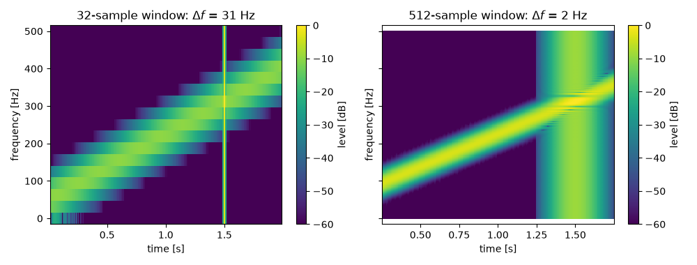
 32-sample window: ridge at t = 1 s is 218.8 Hz (chirp: 225 Hz), 247 frames
512-sample window: ridge at t = 1 s is 224.6 Hz (chirp: 225 Hz), 187 frames