Blackman and Tukey’s spectral windows (1958)

Ralph Blackman and John Tukey’s The Measurement of Power Spectra (1958) turned spectral estimation into an engineering procedure for the telephone and seismic data of the Bell System. Cutting a finite record out of a signal multiplies it by a rectangular window. In frequency, every tone is then smeared by that window’s transform, whose sidelobes fall only slowly, so a strong tone can hide a weak one nearby. Their book named the tapered windows of Julius von Hann and Richard Hamming that trade a wider main lobe for far lower sidelobes (windowed_spectrum()).

import matplotlib.pyplot as plt
import numpy as np

from engineeringkit.signal_processing import db20, windowed_spectrum

Each window’s own spectrum

Zero-padding a constant record shows the window’s transform. The highest sidelobe sets how far below a strong tone a weak one can still be seen.

fs, n = 1.0, 64
expected = {"boxcar": -13.3, "hann": -31.5, "hamming": -42.7, "blackman": -58.1}
fig, axes = plt.subplots(1, 2, figsize=(10, 3.8))
for name, level in expected.items():
    f, magnitude = windowed_spectrum(np.ones(n), fs, window=name, n_fft=64 * n)
    response = db20(np.maximum(magnitude / magnitude[0], 1e-12))
    first_null = np.argmax(np.diff(response) > 0)  # end of the main lobe
    sidelobe = response[first_null:].max()
    print(f"{name:8s}: main lobe half-width {f[first_null] * n:.1f} bins, highest sidelobe {sidelobe:6.1f} dB")
    assert abs(sidelobe - level) < 0.5
    axes[0].plot(f * n, response, label=name)
axes[0].set(xlabel="frequency [bins]", ylabel="gain [dB]", xlim=(0, 16), ylim=(-100, 5), title="Window transforms")
axes[0].legend()

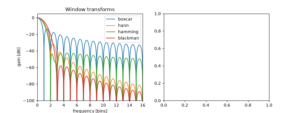
boxcar  : main lobe half-width 1.0 bins, highest sidelobe  -13.3 dB
hann    : main lobe half-width 2.0 bins, highest sidelobe  -31.5 dB
hamming : main lobe half-width 2.0 bins, highest sidelobe  -42.4 dB
blackman: main lobe half-width 3.0 bins, highest sidelobe  -58.1 dB

<matplotlib.legend.Legend object at 0x1110474d0>

A weak tone near a strong one

A tone 50 dB down sits six bins from a strong tone that falls between two bins, the worst case for leakage. The rectangular window buries it; the Blackman window reveals it.

fs, n = 1024.0, 1024
t = np.arange(n) / fs
x = np.sin(2 * np.pi * 100.5 * t) + 10 ** (-50 / 20) * np.sin(2 * np.pi * 107 * t)
visible = {}
for name in ("boxcar", "blackman"):
    f, magnitude = windowed_spectrum(x, fs, window=name)
    level = db20(magnitude / magnitude.max())
    weak = level[np.argmin(abs(f - 107))]
    floor = np.max(level[(f > 104) & (f < 106)])
    visible[name] = weak > floor + 6
    print(f"{name:8s}: weak tone at {weak:6.1f} dB, leakage between the tones {floor:6.1f} dB")
    axes[1].plot(f, level, label=name)
assert not visible["boxcar"] and visible["blackman"]
axes[1].set(xlabel="frequency [Hz]", ylabel="level [dB]", xlim=(85, 125), ylim=(-120, 5), title="Strong tone at 100.5 Hz, weak at 107 Hz")
axes[1].legend()
fig.tight_layout()

plt.show()

boxcar  : weak tone at  -22.5 dB, leakage between the tones  -19.3 dB
blackman: weak tone at  -48.8 dB, leakage between the tones  -58.1 dB