Bogert, Healy and Tukey’s cepstrum (1963)

Seismologists wanted to know how deep an earthquake was, from the delay between a wave and its echo off the surface. An echo multiplies the spectrum by \(1 + \alpha e^{-j\omega d}\): a ripple in the log spectrum whose “frequency” is the delay. Bruce Bogert, Michael Healy and John Tukey (1963) took the spectrum of the log spectrum and found the echo as a peak. They reversed letters to name the new domain: cepstrum, quefrency, liftering. Logarithms turn the convolution of a source and a filter into a sum, which is how pitch is separated from the vocal tract in speech (real_cepstrum()).

import matplotlib.pyplot as plt
import numpy as np
from scipy import signal

from engineeringkit.signal_processing import real_cepstrum

An echo becomes a peak

A coloured pulse and its echo, delayed 37 ms with half the amplitude, at 1 kHz.

fs, delay, alpha = 1000.0, 37, 0.5
rng = np.random.default_rng(1963)
pulse = signal.lfilter([1.0], [1.0, -1.6, 0.8], rng.normal(size=60)) * np.hanning(60)
x = np.zeros(1024)
x[100:160] = pulse
x[100 + delay : 160 + delay] += alpha * pulse
c = real_cepstrum(x)
quefrency = np.arange(c.size) / fs
search = slice(10, 512)
found = (np.argmax(c[search]) + 10) / fs
print(f"cepstral peak at {found * 1e3:.0f} ms, height {c[delay]:.3f} (alpha/2 = {alpha / 2})")
fig, axes = plt.subplots(1, 3, figsize=(13, 3.6))
spectrum = np.abs(np.fft.rfft(x))
axes[0].plot(np.fft.rfftfreq(x.size, 1 / fs), 20 * np.log10(spectrum))
axes[0].set(xlabel="frequency [Hz]", ylabel="log magnitude [dB]", title="Rippled log spectrum")
axes[1].plot(quefrency[1:200] * 1e3, c[1:200])
axes[1].axvline(delay, color="C3", ls="--", lw=0.8)
axes[1].set(xlabel="quefrency [ms]", title="Real cepstrum")

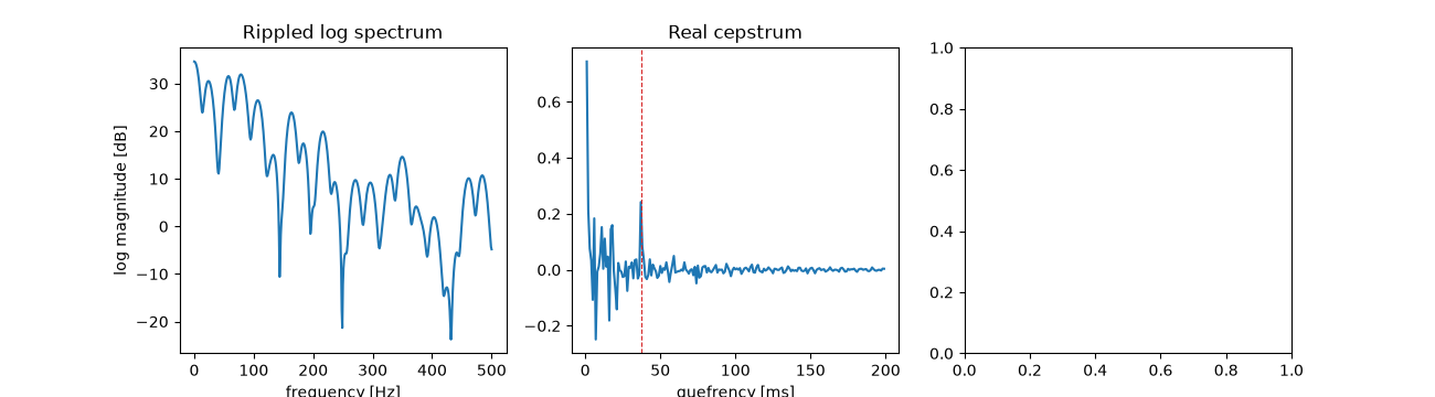
cepstral peak at 37 ms, height 0.242 (alpha/2 = 0.25)

[Text(0.5, 10.433333333333328, 'quefrency [ms]'), Text(0.5, 1.0, 'Real cepstrum')]

Pitch from a pulse train

A crude voiced sound: pulses every 8 ms through a resonance. The cepstrum separates the slowly varying resonance (low quefrency) from the 8 ms pitch period (a peak at 8 ms).

pitch = 8
train = np.zeros(1024)
train[::pitch] = 1.0
voiced = signal.lfilter([1.0], [1.0, -1.3, 0.9], train) + 1e-3 * rng.normal(size=train.size)
cv = real_cepstrum(voiced)
pitch_found = np.argmax(cv[4:100]) + 4
axes[2].plot(quefrency[1:100] * 1e3, cv[1:100])
axes[2].set(xlabel="quefrency [ms]", title=f"Voiced sound: pitch {pitch_found} ms")
fig.tight_layout()
assert np.isclose(found * fs, delay)
assert np.isclose(c[delay], alpha / 2, atol=0.05)
assert pitch_found == pitch

plt.show()