Curzon and Ahlborn: efficiency at maximum power (1975)

A Carnot engine reaches its efficiency only by running infinitely slowly, so it delivers no power. Frank Curzon and Boye Ahlborn (1975), after Novikov and Chambadal (1957), let a reversible engine exchange heat with its reservoirs through finite conductances, \(\dot Q = K\,\Delta T\). Run slowly, it is efficient but weak; run fast, the temperature drops eat the whole temperature difference. At maximum power the efficiency is \(1 - \sqrt{T_c/T_h}\) (curzon_ahlborn_efficiency()), whatever the conductances, and it describes real power plants better than Carnot’s bound does.

import matplotlib.pyplot as plt
import numpy as np
from scipy.optimize import minimize_scalar

from engineeringkit.thermodynamics import carnot_efficiency, curzon_ahlborn_efficiency

Power against the engine’s hot-side temperature

The working fluid takes heat at \(T_{hw} < T_h\) and rejects it at \(T_{cw} > T_c\). The reversible core makes the entropy flows in and out equal, which fixes \(T_{cw}\) for each \(T_{hw}\).

T_h, T_c, K_h, K_c = 838.15, 298.15, 1.0, 1.0  # K, kW/K


def engine(T_hw):
    q_in = K_h * (T_h - T_hw)
    T_cw = K_c * T_c / (K_c - q_in / T_hw)
    eta = 1 - T_cw / T_hw
    return q_in * eta, eta


T_hw = np.linspace(560, T_h - 1e-6, 400)
power, efficiency = np.array([engine(T) for T in T_hw]).T
keep = power >= 0  # below some T_hw the cold side would have to be hotter than the hot side
best = minimize_scalar(lambda T: -engine(T)[0], bounds=(560, T_h), method="bounded", options={"xatol": 1e-8})
P_max, eta_at_max = engine(best.x)
print(f"maximum power {P_max:.1f} kW at efficiency {eta_at_max:.4f}")
print(f"Curzon-Ahlborn {curzon_ahlborn_efficiency(T_h, T_c):.4f}, Carnot {carnot_efficiency(T_h, T_c):.4f}")
assert np.isclose(eta_at_max, curzon_ahlborn_efficiency(T_h, T_c), rtol=1e-6)

fig, ax = plt.subplots(figsize=(6, 3.5))
ax.plot(efficiency[keep], power[keep])
ax.axvline(curzon_ahlborn_efficiency(T_h, T_c), color="C1", ls="--", label="Curzon-Ahlborn")
ax.axvline(carnot_efficiency(T_h, T_c), color="k", ls=":", label="Carnot (zero power)")
ax.set(xlabel="efficiency", ylabel="power [kW]", title="Endoreversible engine, 565 °C to 25 °C")
ax.legend()
fig.tight_layout()

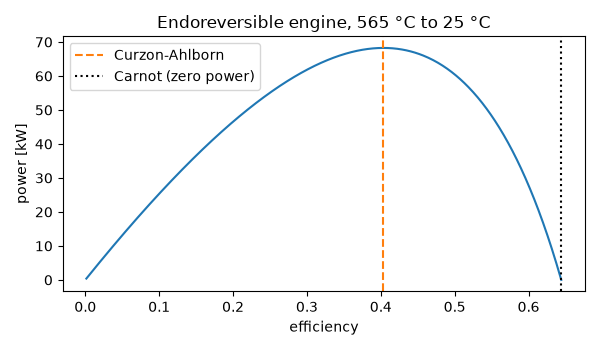
maximum power 68.3 kW at efficiency 0.4036
Curzon-Ahlborn 0.4036, Carnot 0.6443

Real power plants

Curzon and Ahlborn compared their result with three plants, using the observed efficiencies quoted in their paper.

plants = {
    "West Thurrock (coal)": (838.15, 298.15, 0.36),
    "CANDU (nuclear)": (573.15, 298.15, 0.30),
    "Larderello (geothermal)": (523.15, 353.15, 0.16),
}
for name, (Th, Tc, observed) in plants.items():
    ca, carnot = curzon_ahlborn_efficiency(Th, Tc), carnot_efficiency(Th, Tc)
    print(f"{name:24s} observed {observed:.2f}, Curzon-Ahlborn {ca:.3f}, Carnot {carnot:.3f}")
    assert abs(ca - observed) < 0.05 < carnot - observed

plt.show()

West Thurrock (coal)     observed 0.36, Curzon-Ahlborn 0.404, Carnot 0.644
CANDU (nuclear)          observed 0.30, Curzon-Ahlborn 0.279, Carnot 0.480
Larderello (geothermal)  observed 0.16, Curzon-Ahlborn 0.178, Carnot 0.325