Maxwell’s thermodynamic relations (1871)

In his Theory of Heat (1871) James Clerk Maxwell drew a small cycle on the pressure-volume diagram and read off four relations between the derivatives of \(p\), \(v\), \(T\) and \(s\). In modern form they say that the mixed second derivatives of \(u\), \(h\), \(a\) and \(g\) are equal. One of them, \((\partial s/\partial p)_T = -(\partial v/\partial T)_p\), trades an unmeasurable entropy derivative for a measurable expansion coefficient. From it follow the difference of the specific heats (cp_minus_cv()) and the Joule-Thomson coefficient of any fluid (joule_thomson_coefficient()). The example checks both against IAPWS-IF97 steam, which is itself built from a Gibbs function.

import matplotlib.pyplot as plt
import numpy as np

from engineeringkit.thermodynamics import cp_minus_cv, joule_thomson_coefficient, steam_properties

The Maxwell relation on superheated steam

Differentiate IF97 numerically at 2 MPa and 600 K: the entropy lost per pascal of compression equals the volume gained per kelvin of heating.

p, T, dT, dp = 2e6, 600.0, 0.01, 100.0
ds_dp = (steam_properties(p + dp, T).s - steam_properties(p - dp, T).s) / (2 * dp)
dv_dT = (steam_properties(p, T + dT).v - steam_properties(p, T - dT).v) / (2 * dT)
print(f"(ds/dp)_T = {ds_dp:.6e} m³/(kg K);  -(dv/dT)_p = {-dv_dT:.6e} m³/(kg K)")
assert np.isclose(ds_dp, -dv_dT, rtol=1e-5)

(ds/dp)_T = -2.610761e-04 m³/(kg K);  -(dv/dT)_p = -2.610761e-04 m³/(kg K)

Two consequences

The expansivity \(\beta\) and compressibility \(\kappa_T\) give \(c_p - c_v = Tv\beta^2/\kappa_T\), which is \(R\) for an ideal gas, and \(\mu_{JT} = v(T\beta - 1)/c_p\), which is zero for one.

st = steam_properties(p, T)
beta = dv_dT / st.v
kappa = -(steam_properties(p + dp, T).v - steam_properties(p - dp, T).v) / (2 * dp) / st.v
mu = joule_thomson_coefficient(T, st.v, beta, st.cp)
throttled = steam_properties(p - 10e3, h=st.h)
print(f"cp - cv = {cp_minus_cv(T, st.v, beta, kappa):.1f} J/(kg K) (ideal steam: 461.5)")
print(f"Joule-Thomson coefficient {mu * 1e6:.3f} K/MPa; a 10 kPa throttle cools by {(T - throttled.T) * 1e3:.2f} mK")
assert np.isclose((T - throttled.T) / 10e3, mu, rtol=2e-3)

cp - cv = 589.5 J/(kg K) (ideal steam: 461.5)
Joule-Thomson coefficient 10.630 K/MPa; a 10 kPa throttle cools by 106.33 mK

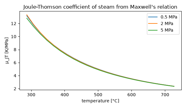
Across the vapour region the coefficient falls towards zero as the steam approaches an ideal gas at high temperature and low pressure.

temps = np.linspace(560.0, 1000.0, 23)  # above the 537 K boiling point at 5 MPa
fig, ax = plt.subplots(figsize=(6, 3.5))
for pressure in (0.5e6, 2e6, 5e6):
    values = []
    for Ti in temps:
        here = steam_properties(pressure, Ti)
        b = (steam_properties(pressure, Ti + dT).v - steam_properties(pressure, Ti - dT).v) / (2 * dT) / here.v
        values.append(joule_thomson_coefficient(Ti, here.v, b, here.cp) * 1e6)
    ax.plot(temps - 273.15, values, label=f"{pressure / 1e6:g} MPa")
ax.set(xlabel="temperature [°C]", ylabel="μ_JT [K/MPa]", title="Joule-Thomson coefficient of steam from Maxwell's relation")
ax.legend()
fig.tight_layout()
assert values[0] > values[-1] > 0

plt.show()