Joule’s first law in steady-flow devices (1843-1850)

Joule’s equivalence of heat and work, written for fluid flowing steadily through a device, is the energy balance of every engineering component:

\[q - w = (h_2 - h_1) + \tfrac12(V_2^2 - V_1^2) + g(z_2 - z_1)\]

(steady_flow_work()). A nozzle turns enthalpy into speed (nozzle_exit_velocity()). A turbine turns it into shaft work, a throttle keeps it (throttle_steam()) and a mixing chamber averages it (mixing_chamber()). Real turbines and compressors are rated against the isentropic device (turbine_isentropic_efficiency()).

import matplotlib.pyplot as plt
import numpy as np

from engineeringkit.thermodynamics import (
    expansion_outlet_enthalpy,
    mixing_chamber,
    nozzle_exit_velocity,
    steady_flow_work,
    steam_properties,
    throttle_steam,
    turbine_isentropic_efficiency,
)

A steam turbine and its isentropic efficiency

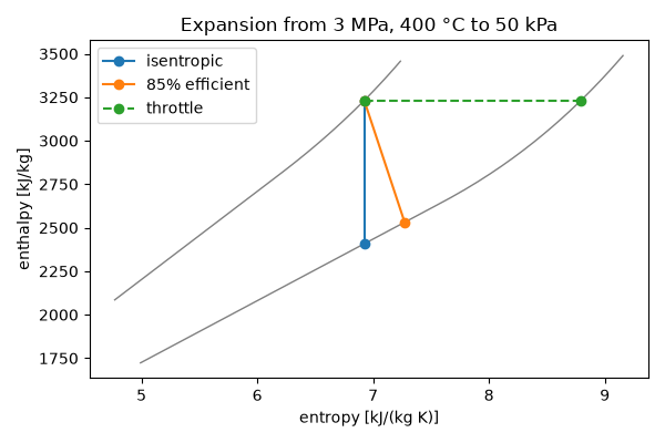
Steam enters at 3 MPa and 400 °C and leaves at 50 kPa. The isentropic expansion sets the ideal work; an 85% efficient turbine delivers less and leaves drier, higher-entropy steam.

inlet = steam_properties(3e6, 673.15)
ideal = steam_properties(50e3, s=inlet.s)
real = steam_properties(50e3, h=expansion_outlet_enthalpy(inlet.h, ideal.h, 0.85))
w_ideal, w_real = steady_flow_work(inlet.h, ideal.h), steady_flow_work(inlet.h, real.h)
print(f"ideal work {w_ideal / 1e3:.1f} kJ/kg (exit quality {ideal.x:.3f}); real work {w_real / 1e3:.1f} kJ/kg (quality {real.x:.3f})")
print(f"entropy generated {(real.s - inlet.s):.1f} J/(kg K)")
assert np.isclose(turbine_isentropic_efficiency(inlet.h, real.h, ideal.h), 0.85) and real.s > inlet.s

ideal work 823.7 kJ/kg (exit quality 0.897); real work 700.2 kJ/kg (quality 0.951)
entropy generated 348.6 J/(kg K)

A nozzle, a throttle and a mixing chamber

The same enthalpy drop in an adiabatic nozzle accelerates the steam instead; a throttle from the same inlet keeps the enthalpy and only loses pressure and work potential; a feedwater heater mixes hot and cold streams.

V = nozzle_exit_velocity(inlet.h, steam_properties(2e6, s=inlet.s).h, V_in=40.0)
throttled = throttle_steam(inlet, 50e3)
print(f"nozzle to 2 MPa: {V:.0f} m/s; throttle to 50 kPa: {throttled.T - 273.15:.1f} °C, entropy +{throttled.s - inlet.s:.0f} J/(kg K)")
hot, cold = steam_properties(200e3, 473.15), steam_properties(200e3, 293.15)
target = steam_properties(200e3, x=0.0).h
y = (target - cold.h) / (hot.h - cold.h)
m_out, h_out = mixing_chamber([y, 1 - y], [hot.h, cold.h])
print(f"saturated liquid at 200 kPa needs {y:.3f} kg of 200 °C steam per kg of outlet water")
assert np.isclose(steady_flow_work(inlet.h, throttled.h), 0) and np.isclose(h_out, target)

nozzle to 2 MPa: 482 m/s; throttle to 50 kPa: 376.8 °C, entropy +1870 J/(kg K)
saturated liquid at 200 kPa needs 0.151 kg of 200 °C steam per kg of outlet water

The turbine on the h-s (Mollier) diagram

fig, ax = plt.subplots(figsize=(6, 4))
for p in (3e6, 50e3):
    path = steam_properties(p, h=np.linspace(steam_properties(p, x=0.6).h, steam_properties(p, 773.15).h, 40))
    ax.plot(path.s / 1e3, path.h / 1e3, color="gray", lw=1)
ax.plot([inlet.s / 1e3, ideal.s / 1e3], [inlet.h / 1e3, ideal.h / 1e3], "o-", label="isentropic")
ax.plot([inlet.s / 1e3, real.s / 1e3], [inlet.h / 1e3, real.h / 1e3], "o-", label="85% efficient")
ax.plot([inlet.s / 1e3, throttled.s / 1e3], [inlet.h / 1e3, throttled.h / 1e3], "o--", label="throttle")
ax.set(xlabel="entropy [kJ/(kg K)]", ylabel="enthalpy [kJ/kg]", title="Expansion from 3 MPa, 400 °C to 50 kPa")
ax.legend()
fig.tight_layout()
assert w_real < w_ideal

plt.show()