IAPWS-IF97: the properties of water and steam (1997)

Steam tables have been the working data of power engineering since Callendar and Mollier’s tables of the early 1900s. In 1997 the International Association for the Properties of Water and Steam adopted the Industrial Formulation IAPWS-IF97, led by Wolfgang Wagner. It splits the fluid into five regions, each with its own fast equation fitted to the scientific formulation IAPWS-95. In the compressed liquid (region 1) and the vapour (region 2) the equation is a dimensionless Gibbs free energy \(g(p, T)/(RT)\), and every property follows from its derivatives. Near the critical point (region 3) it is a Helmholtz free energy \(f(\rho, T)/(RT)\) of density, and region 4 is the saturation line (steam_properties(), saturation_pressure()). The example checks the release’s own verification values and draws the T-s diagram.

import matplotlib.pyplot as plt
import numpy as np

from engineeringkit.thermodynamics import saturation_pressure, saturation_temperature, steam_properties
from engineeringkit.thermodynamics.utils import if97
from engineeringkit.thermodynamics.visualizers import plot_saturation_dome

The verification values

The release gives property values to nine digits so that every implementation can be checked. Two from Tables 5 and 15:

checks = [
    (3e6, 300.0, 0.100215168e-2, 0.115331273e3, 0.392294792),  # region 1
    (0.0035e6, 700.0, 0.923015898e2, 0.333568375e4, 0.101749996e2),  # region 2
]
for p, T, v, h, s in checks:
    st = steam_properties(p, T)
    print(f"region {st.region}: p = {p / 1e6:g} MPa, T = {T:g} K")
    print(f"  v = {st.v:.9e} m³/kg, h = {st.h / 1e3:.6f} kJ/kg, s = {st.s / 1e3:.9f} kJ/(kg K)")
    np.testing.assert_allclose((st.v, st.h / 1e3, st.s / 1e3), (v, h, s), rtol=1e-8)
np.testing.assert_allclose(saturation_pressure(500.0), 0.263889776e7, rtol=1e-8)
np.testing.assert_allclose(saturation_temperature(1e6), 0.453035632e3, rtol=1e-8)

region 1: p = 3 MPa, T = 300 K
  v = 1.002151680e-03 m³/kg, h = 115.331273 kJ/kg, s = 0.392294792 kJ/(kg K)
region 2: p = 0.0035 MPa, T = 700 K
  v = 9.230158982e+01 m³/kg, h = 3335.683754 kJ/kg, s = 10.174999579 kJ/(kg K)

Region 3 is given in density, so its check (Table 33) is at a density and temperature. steam_properties goes the other way: from pressure and temperature it solves the Helmholtz pressure for the density.

props = if97.region3(500.0, 650.0)
print(f"region 3: rho = 500 kg/m³, T = 650 K: p = {props['p'] / 1e6:.7f} MPa, h = {props['h'] / 1e3:.5f} kJ/kg")
np.testing.assert_allclose((props["p"] / 1e6, props["h"] / 1e3), (25.5837018, 1863.43019), rtol=1e-8)
st = steam_properties(float(props["p"]), 650.0)
assert st.region == 3 and abs(1 / st.v - 500.0) < 1e-6

region 3: rho = 500 kg/m³, T = 650 K: p = 25.5837018 MPa, h = 1863.43019 kJ/kg

How ideal is steam?

The compressibility \(Z = pv/(RT)\) is one for an ideal gas. Low-pressure steam, as in the air or a condenser, is close to ideal. Boiler steam is not, which is why the ideal gas laws cannot be used for steam cycles.

for p, T in ((3.5e3, 300.0), (101325.0, 400.0), (10e6, 773.15), (16e6, 623.15)):
    st = steam_properties(p, T)
    Z = p * st.v / (if97.R_WATER * T)
    print(f"p = {p / 1e6:8.4f} MPa, T = {T - 273.15:6.1f} °C: Z = {Z:.4f}")
assert abs(steam_properties(3.5e3, 300.0).v * 3.5e3 / (if97.R_WATER * 300.0) - 1) < 2e-3
assert steam_properties(16e6, 623.15).v * 16e6 / (if97.R_WATER * 623.15) < 0.75

p =   0.0035 MPa, T =   26.9 °C: Z = 0.9983
p =   0.1013 MPa, T =  126.9 °C: Z = 0.9891
p =  10.0000 MPa, T =  500.0 °C: Z = 0.9196
p =  16.0000 MPa, T =  350.0 °C: Z = 0.5433

The T-s diagram

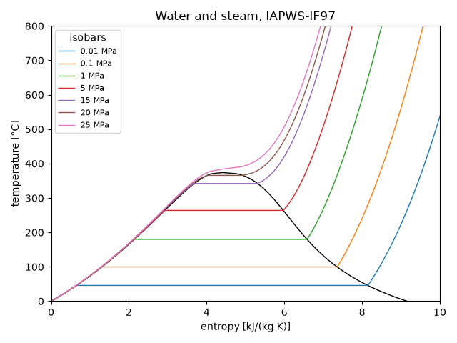
Under the dome liquid and vapour coexist at the saturation temperature, so isobars are horizontal there. The dome closes at the critical point, 374 °C and 22.064 MPa; the 25 MPa isobar passes above it, so the fluid goes from liquid to vapour with no boiling at all.

ax = plot_saturation_dome()
for p in (10e3, 0.1e6, 1e6, 5e6, 15e6, 20e6, 25e6):
    if p > if97.P_CRIT:
        path = [steam_properties(p, T) for T in np.linspace(275.0, 1073.15, 120)]
    else:
        T_sat = float(saturation_temperature(p))
        liquid = [steam_properties(p, T) for T in np.linspace(275.0, T_sat - 0.01, 40)]
        wet = [steam_properties(p, x=x) for x in np.linspace(0, 1, 10)]
        vapour = [steam_properties(p, T) for T in np.linspace(T_sat + 0.01, 1073.15, 60)]
        path = liquid + wet + vapour
    ax.plot([st.s / 1e3 for st in path], [st.T - 273.15 for st in path], lw=1, label=f"{p / 1e6:g} MPa")
    entropies = [st.s for st in path]
    assert np.all(np.diff(entropies) > 0)  # entropy rises with heat added along an isobar
ax.set(title="Water and steam, IAPWS-IF97", xlim=(0, 10), ylim=(0, 800))
ax.legend(fontsize=8, title="isobars")
ax.figure.tight_layout()

plt.show()