Peng and Robinson’s equation of state (1976)

Ding-Yu Peng and Donald Robinson, at the University of Alberta, wanted one simple equation for the vapour-liquid equilibria of natural gas. They kept van der Waals’s two terms but changed the attraction’s volume dependence and made it fall with temperature through the acentric factor:

\[p = \frac{RT}{v - b} - \frac{a\alpha(T)}{v^2 + 2bv - b^2}\]

(peng_robinson_pressure()). The critical compressibility becomes 0.307 instead of 3/8. Equal liquid and vapour fugacities give the vapour pressure (peng_robinson_saturation_pressure()). Three constants then describe a refrigerant well enough to design with (refrigerant_properties()).

import matplotlib.pyplot as plt
import numpy as np

from engineeringkit.thermodynamics import (
    R134A,
    R_UNIVERSAL,
    peng_robinson_compressibility,
    peng_robinson_pressure,
    peng_robinson_saturation_pressure,
    refrigerant_properties,
)

fluid = R134A

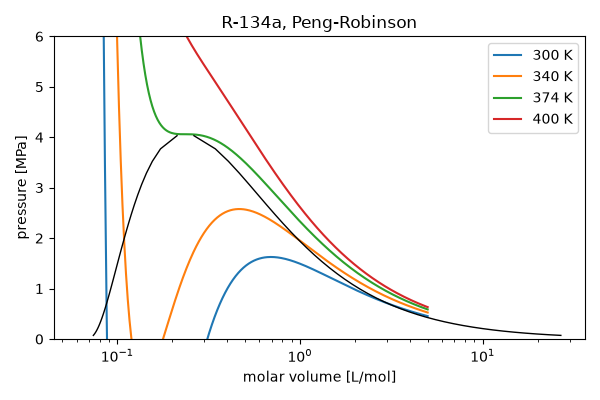
Isotherms and the saturation dome of R-134a

Below the critical temperature each isotherm has a loop; the saturation pressure cuts it into equal areas, Maxwell’s rule.

fig, ax = plt.subplots(figsize=(6, 4))
v = np.geomspace(1.02 * 0.0778 * R_UNIVERSAL * fluid.Tc / fluid.pc, 5e-3, 400)
for T in (300.0, 340.0, fluid.Tc, 400.0):
    ax.plot(v * 1e3, peng_robinson_pressure(T, v, fluid.Tc, fluid.pc, fluid.omega) / 1e6, label=f"{T:.0f} K")
dome_T = np.linspace(240.0, 0.999 * fluid.Tc, 40)
dome_p = np.array([peng_robinson_saturation_pressure(T, fluid.Tc, fluid.pc, fluid.omega) for T in dome_T])
for phase in ("liquid", "vapour"):
    z = [peng_robinson_compressibility(T, p, fluid.Tc, fluid.pc, fluid.omega, phase=phase) for T, p in zip(dome_T, dome_p)]
    ax.plot(np.array(z) * R_UNIVERSAL * dome_T / dome_p * 1e3, dome_p / 1e6, "k-", lw=1)
ax.set(xscale="log", ylim=(0, 6), xlabel="molar volume [L/mol]", ylabel="pressure [MPa]", title="R-134a, Peng-Robinson")
ax.legend()
fig.tight_layout()

Against the refrigerant tables

Çengel and Boles, Table A-11 (from the reference equation of state): the vapour pressure and the latent heat at three temperatures.

table = {-40: (51.25e3, 225.86e3), 0: (293.01e3, 198.60e3), 40: (1017.1e3, 163.02e3)}
for T_c, (p_table, hfg_table) in table.items():
    T = T_c + 273.15
    p = peng_robinson_saturation_pressure(T, fluid.Tc, fluid.pc, fluid.omega)
    hfg = refrigerant_properties(fluid, p, x=1.0).h - refrigerant_properties(fluid, p, x=0.0).h
    print(f"{T_c:+d} °C: p_sat {p / 1e3:7.1f} kPa (table {p_table / 1e3:7.1f}), h_fg {hfg / 1e3:5.1f} kJ/kg (table {hfg_table / 1e3:5.1f})")
    assert np.isclose(p, p_table, rtol=0.02) and np.isclose(hfg, hfg_table, rtol=0.04)

zc = 0.3074
print(f"critical compressibility {zc} (van der Waals 0.375, R-134a measured about 0.26)")

plt.show()

-40 °C: p_sat    51.4 kPa (table    51.2), h_fg 225.5 kJ/kg (table 225.9)
+0 °C: p_sat   291.8 kPa (table   293.0), h_fg 201.6 kJ/kg (table 198.6)
+40 °C: p_sat  1017.0 kPa (table  1017.1), h_fg 166.9 kJ/kg (table 163.0)
critical compressibility 0.3074 (van der Waals 0.375, R-134a measured about 0.26)