Carrier’s psychrometric chart (1911)

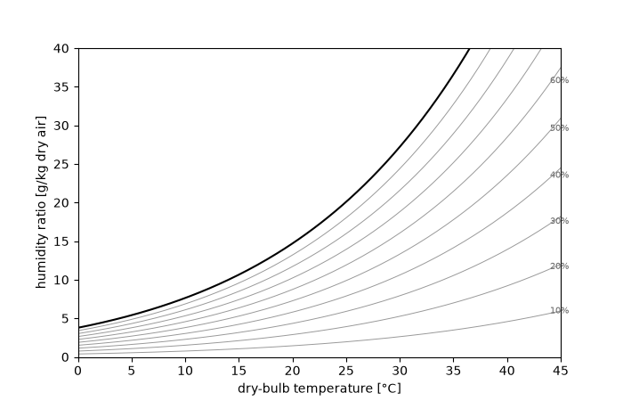
In 1902 Willis Carrier designed a system to control the humidity in a Brooklyn printing plant, where paper swelling in the summer air spoiled the colour registration. He cooled the air below its dew point to condense the excess water, then let it warm up again. His 1911 paper “Rational psychrometric formulae” treated moist air as an ideal mixture of dry air and water vapour and drew the chart that air-conditioning engineers still use: humidity ratio \(w = 0.622\,p_v/(p - p_v)\) (humidity_ratio()) against dry-bulb temperature, with curves of constant relative humidity (relative_humidity()) and the dew point (dew_point()) where they meet saturation.

import matplotlib.pyplot as plt
import numpy as np

from engineeringkit.thermodynamics import dew_point, humidity_ratio, relative_humidity

The chart

T = np.linspace(273.15, 318.15, 200)
fig, ax = plt.subplots(figsize=(7, 4.5))
for phi in np.arange(0.1, 1.01, 0.1):
    ax.plot(T - 273.15, humidity_ratio(T, phi) * 1e3, color="k" if phi > 0.99 else "0.6", lw=1.5 if phi > 0.99 else 0.7)
    ax.annotate(f"{phi:.0%}", (44, humidity_ratio(317.15, phi) * 1e3), fontsize=7, color="0.4")
ax.set(xlabel="dry-bulb temperature [°C]", ylabel="humidity ratio [g/kg dry air]", xlim=(0, 45), ylim=(0, 40))

[Text(0.5, 20.33333333333333, 'dry-bulb temperature [°C]'), Text(54.222222222222214, 0.5, 'humidity ratio [g/kg dry air]'), (0.0, 45.0), (0.0, 40.0)]

Carrier’s process

Summer air at 32 °C and 60% relative humidity is cooled. Its humidity ratio stays the same until it reaches the dew point, 23 °C. Below that, water condenses and the air follows the saturation curve down to 12 °C. Reheating to 22 °C gives comfortable air at about half the relative humidity.

T_in, phi_in, T_coil, T_supply = 305.15, 0.60, 285.15, 295.15
w_in = humidity_ratio(T_in, phi_in)
T_dew = dew_point(w_in)
w_coil = humidity_ratio(T_coil, 1.0)
phi_supply = relative_humidity(T_supply, w_coil)
condensate = w_in - w_coil
print(f"inlet: w = {w_in * 1e3:.2f} g/kg, dew point {T_dew - 273.15:.1f} °C")
print(f"after the coil at 12 °C: w = {w_coil * 1e3:.2f} g/kg; condensate {condensate * 1e3:.2f} g per kg of dry air")
print(f"supply at 22 °C: relative humidity {phi_supply:.0%}")
assert np.isclose(relative_humidity(T_dew, w_in), 1.0)
assert np.isclose(relative_humidity(T_in, w_in), phi_in)
assert 0.45 < phi_supply < 0.6 and condensate > 0

T_sat_path = np.linspace(T_dew, T_coil, 30)
process_T = np.concatenate([[T_in, T_dew], T_sat_path, [T_supply]]) - 273.15
process_w = np.concatenate([[w_in, w_in], humidity_ratio(T_sat_path, 1.0), [w_coil]]) * 1e3
ax.plot(process_T, process_w, "C3-", lw=2)
for label, Tp, wp in (("inlet", T_in, w_in), ("dew point", T_dew, w_in), ("coil", T_coil, w_coil), ("supply", T_supply, w_coil)):
    ax.plot(Tp - 273.15, wp * 1e3, "o", color="C3")
    ax.annotate(label, (Tp - 273.15, wp * 1e3), textcoords="offset points", xytext=(4, 4), fontsize=8)
ax.set_title("Psychrometric chart at sea level: cooling, dehumidifying, reheating")
fig.tight_layout()

inlet: w = 18.04 g/kg, dew point 23.3 °C
after the coil at 12 °C: w = 8.73 g/kg; condensate 9.30 g per kg of dry air
supply at 22 °C: relative humidity 53%

The condensate is real water that the cooling coil must drain: a building supplied with 10 kg/s of this air removes about 330 litres an hour. Taking it out also takes the latent heat of condensation, about 2.45 MJ per kilogram, so a large part of an air conditioner’s load in humid climates goes to drying the air, not cooling it.

litres_per_hour = 10.0 * condensate * 3600
print(f"condensate at 10 kg/s of dry air: {litres_per_hour:.0f} L/h")
assert 300 < litres_per_hour < 420

plt.show()

condensate at 10 kg/s of dry air: 335 L/h