Kelvin’s heat pump (1852)

In 1852 William Thomson, later Lord Kelvin, pointed out that the second law cuts both ways. A refrigerator run backwards would warm a building with heat drawn from the cold outside air, and the heat delivered would be many times the work spent. He proposed an air machine for it: compress outside air, let it give its heat to the rooms, then expand it. The figure of merit is \(\mathrm{COP}_{HP} = Q_h/W\) (heat_pump_cop()), at most \(T_h/(T_h - T_c)\) (carnot_cop_heat_pump()). Practical heat pumps had to wait for vapour compression and cheap electricity; they now heat millions of homes.

import matplotlib.pyplot as plt
import numpy as np

from engineeringkit.thermodynamics import (
    brayton_efficiency,
    carnot_cop_heat_pump,
    carnot_cop_refrigerator,
    heat_pump_cop,
    isentropic_temperature_ratio,
)

Kelvin’s air machine

Outside air at 2 °C is compressed through a pressure ratio \(r_p\), gives up heat until it reaches the room temperature of 20 °C, is expanded back to atmospheric pressure (now colder than outside), and is warmed by the outside air again. This is the Brayton cycle run backwards, so its COP is \(1/\eta_{Brayton}\).

cp, T_out, T_room = 1005.0, 275.15, 293.15
for rp in (1.3, 1.5, 2.0):
    tau = isentropic_temperature_ratio(rp)
    T_supply, T_exhaust = T_out * tau, T_room / tau
    q_hot = cp * (T_supply - T_room)
    w = q_hot - cp * (T_out - T_exhaust)
    cop = heat_pump_cop(q_hot, w)
    print(f"r_p = {rp}: air leaves the compressor at {T_supply - 273.15:5.1f} °C, COP = {cop:.2f}")
    assert np.isclose(cop, 1 / brayton_efficiency(rp))
cop_max = carnot_cop_heat_pump(T_room, T_out)
print(f"Carnot COP between 2 °C and 20 °C: {cop_max:.1f}")
assert 1 / brayton_efficiency(1.3) < cop_max

r_p = 1.3: air leaves the compressor at  23.4 °C, COP = 13.85
r_p = 1.5: air leaves the compressor at  35.8 °C, COP = 9.14
r_p = 2.0: air leaves the compressor at  62.3 °C, COP = 5.57
Carnot COP between 2 °C and 20 °C: 16.3

The air cycle delivers its heat over a range of temperatures, all of it hotter than the room, so it falls short of Carnot. Still, at a pressure ratio of 1.3 it gives nearly 14 units of heat for each unit of work.

A refrigerator and a heat pump are the same machine

By the first law \(Q_h = Q_c + W\), so \(\mathrm{COP}_{HP} = \mathrm{COP}_R + 1\). A real heat pump reaches about half of Carnot.

T_outside = np.linspace(253.15, 288.15, 50)
cop_carnot = np.array([carnot_cop_heat_pump(308.15, T) for T in T_outside])
assert np.allclose(cop_carnot, [carnot_cop_refrigerator(308.15, T) + 1 for T in T_outside])
cop_real = 0.5 * cop_carnot

Kelvin’s economy argument

Burning fuel in a boiler gives at most one joule of heat per joule of fuel. Burning it in a power station of efficiency 0.40 and driving a heat pump gives \(0.40\,\mathrm{COP}\) joules of heat, even if the station’s own waste heat is thrown away. With underfloor heating at 35 °C, the heat pump beats the boiler even at -20 °C.

eta_plant, eta_boiler = 0.40, 0.90
heat_per_fuel = eta_plant * cop_real
fig, axes = plt.subplots(1, 2, figsize=(10, 3.8))
axes[0].plot(T_outside - 273.15, cop_carnot, "--", label="Carnot")
axes[0].plot(T_outside - 273.15, cop_real, label="real (half of Carnot)")
axes[0].set(xlabel="outside temperature [°C]", ylabel="COP", title="Heating water to 35 °C")
axes[0].legend()
axes[1].plot(T_outside - 273.15, heat_per_fuel, label="power station + heat pump")
axes[1].axhline(eta_boiler, color="C3", ls=":", label="condensing boiler")
axes[1].set(xlabel="outside temperature [°C]", ylabel="heat delivered per unit of fuel")
axes[1].legend()
fig.tight_layout()
assert np.all(heat_per_fuel > eta_boiler)
print(f"at -20 °C: COP {cop_real[0]:.2f}, heat per unit of fuel {heat_per_fuel[0]:.2f} against {eta_boiler} for a boiler")

plt.show()

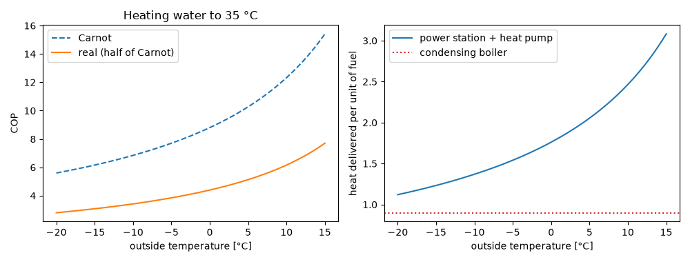
at -20 °C: COP 2.80, heat per unit of fuel 1.12 against 0.9 for a boiler