Hartley’s law: information grows with the logarithm of the levels

Ralph Hartley (1928) argued that a message selected from \(M\) distinguishable symbols carries \(\log M\) units of information, so a channel of bandwidth \(B\) carrying \(2B\) symbols per second has a line rate of \(2B\log_2 M\) bits per second (hartley_capacity()). More levels raise the rate only logarithmically, and noise limits how many levels can be told apart. This example sends multilevel symbols through a noisy channel to show that limit.

import matplotlib.pyplot as plt
import numpy as np

from engineeringkit.communications import hartley_capacity, symbol_rate

Line rate of a 3 kHz telephone channel

B = 3000.0
for M in [2, 4, 8, 16, 64]:
    rate = float(hartley_capacity(B, M))
    print(f"M = {M:2d}: {rate:7.0f} bit/s at {float(symbol_rate(rate, M)):.0f} baud")

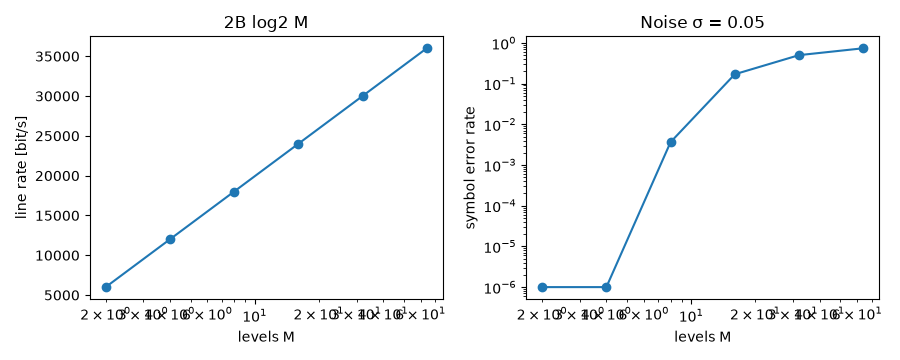
M =  2:    6000 bit/s at 6000 baud
M =  4:   12000 bit/s at 6000 baud
M =  8:   18000 bit/s at 6000 baud
M = 16:   24000 bit/s at 6000 baud
M = 64:   36000 bit/s at 6000 baud

Noise sets how many levels survive

Equally spaced levels in [-1, 1] with Gaussian noise of standard deviation 0.05: the symbol error rate jumps once the level spacing approaches the noise.

rng = np.random.default_rng(1928)
levels = [2, 4, 8, 16, 32, 64]
errors = []
for M in levels:
    alphabet = np.linspace(-1, 1, M)
    sent = rng.integers(0, M, 50_000)
    received = alphabet[sent] + rng.normal(0, 0.05, sent.size)
    decided = np.argmin(np.abs(received[:, None] - alphabet[None, :]), axis=1)
    errors.append(np.mean(decided != sent))
fig, axes = plt.subplots(1, 2, figsize=(9, 3.6))
axes[0].plot(levels, [float(hartley_capacity(B, m)) for m in levels], "o-")
axes[0].set(xscale="log", xlabel="levels M", ylabel="line rate [bit/s]", title="2B log2 M")
axes[1].semilogy(levels, np.maximum(errors, 1e-6), "o-")
axes[1].set(xscale="log", xlabel="levels M", ylabel="symbol error rate", title="Noise σ = 0.05")
fig.tight_layout()
assert errors[0] < 1e-3 < errors[-1]

plt.show()