Bode’s sensitivity integral (1945)

Hendrik Bode defined the sensitivity of a feedback loop, \(S = 1/(1 + L)\), as the fraction of a plant change that survives in the closed loop (sensitivity()), and its complement \(T = L/(1 + L)\) (complementary_sensitivity()) as the map from reference and sensor noise to the output. Since \(S + T = 1\), the two cannot both be small at one frequency. Bode also showed that, for a stable loop that rolls off at least as \(1/s^2\), \(\int_0^\infty \ln|S(j\omega)|\,d\omega = 0\). Sensitivity pushed down at low frequency pops up elsewhere, the waterbed effect. Freudenberg and Looze (1985) showed that each unstable open-loop pole \(p\) raises the integral to \(\pi\sum \mathrm{Re}\,p\).

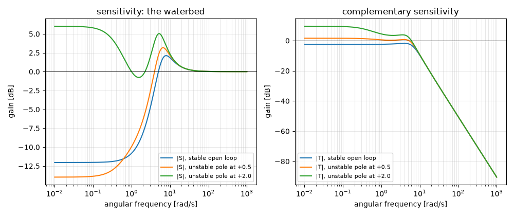
p = -1.0: integral -0.0000 (pi * max(p, 0) = 0.0000), Ms = 1.28, PM 75.9 >= 46.1 deg
p = +0.5: integral 1.5708 (pi * max(p, 0) = 1.5708), Ms = 1.44, PM 55.1 >= 40.6 deg
p = +2.0: integral 6.2832 (pi * max(p, 0) = 6.2832), Ms = 2.00, PM 37.8 >= 29.0 deg

import matplotlib.pyplot as plt
import numpy as np
from scipy import integrate

from engineeringkit.control_systems import (
    complementary_sensitivity,
    nyquist,
    poles,
    sensitivity,
    sensitivity_peak,
    stability_margins,
    transfer_function,
)

w = np.logspace(-2, 3, 2000)
fig, axs = plt.subplots(1, 2, figsize=(10, 4.2))
for p in (-1.0, 0.5, 2.0):
    loop = transfer_function([30, 30], np.polymul([1, -p], [1, 7, 10]))  # 30 (s+1) / ((s-p)(s+2)(s+5))
    S, T = sensitivity(loop), complementary_sensitivity(loop)
    assert np.all(poles(S).real < 0)
    s, t = nyquist(S, w), nyquist(T, w)
    assert np.allclose(s + t, 1)

    def integrand(x):
        return np.log(abs(1 / (1 + nyquist(loop, x))))

    value = sum(integrate.quad(integrand, a, b, limit=400)[0] for a, b in [(0, 1), (1, 100), (100, np.inf)])
    peak, margins = sensitivity_peak(loop), stability_margins(loop)
    print(
        f"p = {p:+.1f}: integral {value:.4f} (pi * max(p, 0) = {np.pi * max(p, 0):.4f}), Ms = {peak['Ms']:.2f}, "
        f"PM {margins['phase_margin_deg']:.1f} >= {peak['phase_margin_bound_deg']:.1f} deg"
    )
    assert abs(value - np.pi * max(p, 0)) < 2e-4
    assert margins["phase_margin_deg"] >= peak["phase_margin_bound_deg"]
    label = "stable open loop" if p < 0 else f"unstable pole at +{p}"
    (line,) = axs[0].semilogx(w, 20 * np.log10(np.abs(s)), label=f"|S|, {label}")
    axs[1].semilogx(w, 20 * np.log10(np.abs(t)), color=line.get_color(), label=f"|T|, {label}")

for ax, title in zip(axs, ("sensitivity: the waterbed", "complementary sensitivity")):
    ax.axhline(0, color="k", lw=0.6)
    ax.set(xlabel="angular frequency [rad/s]", ylabel="gain [dB]", title=title)
    ax.grid(True, which="both", alpha=0.3)
    ax.legend(fontsize=8)
fig.tight_layout()
plt.show()