Fourier’s Théorie analytique de la chaleur (1822)

Joseph Fourier’s 1822 treatise made the heat flux proportional to the temperature gradient, \(q = -k\,\mathrm{d}T/\mathrm{d}x\), derived the heat equation from it, and invented the series that bear his name to solve it. For steady flow through a slab the law gives \(\dot Q = kA\Delta T/L\) (fourier_heat_rate()), so a slab behaves like an electrical resistor \(L/(kA)\) (plane_wall_resistance()) and layered walls add like resistors in series (composite_wall()). Curved walls give logarithmic resistances, and with them the surprising critical radius of insulation.

import matplotlib.pyplot as plt
import numpy as np
from scipy.optimize import minimize_scalar

from engineeringkit.heat_transfer import (
    composite_wall,
    convection_resistance,
    critical_insulation_radius_cylinder,
    critical_insulation_radius_sphere,
    cylinder_resistance,
    fourier_heat_rate,
    overall_u,
    plane_wall_resistance,
    sphere_resistance,
)

A furnace wall as a resistor chain

Firebrick, insulating brick and steel casing, 1 m², with a hot gas film inside and still air outside.

layers = [(0.20, 1.4), (0.10, 0.15), (0.006, 45.0)]  # (thickness m, k W/(m K)), hot side first
wall = composite_wall(1400.0, 300.0, layers, A=1.0, h_hot=60.0, h_cold=12.0)
print(f"heat loss {wall.heat_rate:.0f} W/m²; node temperatures [K]: {np.round(wall.interface_temperatures, 1)}")

# Each layer obeys Fourier's law with its own temperature drop.
for i, (L, k) in enumerate(layers, start=1):
    drop = wall.interface_temperatures[i] - wall.interface_temperatures[i + 1]
    assert np.isclose(fourier_heat_rate(k, 1.0, drop, L), wall.heat_rate)
R = [convection_resistance(60.0)] + [plane_wall_resistance(L, k) for L, k in layers] + [convection_resistance(12.0)]
assert np.isclose(overall_u(*R) * 1100.0, wall.heat_rate)
print("Fourier's law holds layer by layer; the conductance 1/sum(R) gives the same heat rate")

fig, axes = plt.subplots(1, 2, figsize=(10, 3.8))
x = np.concatenate([[0.0], np.cumsum([L for L, _ in layers])])
axes[0].plot(x * 100, wall.interface_temperatures[1:-1], "o-")
axes[0].set(xlabel="depth into wall [cm]", ylabel="temperature [K]", title="Straight lines in each layer")

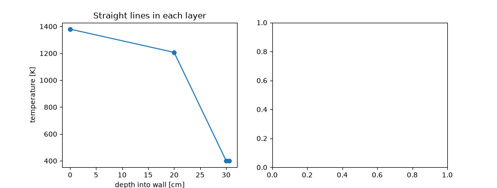
heat loss 1209 W/m²; node temperatures [K]: [1400.  1379.8 1207.1  400.9  400.8  300. ]
Fourier's law holds layer by layer; the conductance 1/sum(R) gives the same heat rate

[Text(0.5, 12.633333333333331, 'depth into wall [cm]'), Text(73.72222222222221, 0.5, 'temperature [K]'), Text(0.5, 1.0, 'Straight lines in each layer')]

Insulating a thin wire

Around a cylinder, conduction resistance \(\ln(r/r_i)/(2\pi kL)\) grows slowly with the outer radius while the convection resistance \(1/(2\pi r h L)\) falls. Their sum is smallest, and the heat loss largest, at \(r_{cr} = k/h\).

k_ins, h, r_wire = 0.17, 8.0, 0.002  # PVC on a 4 mm wire in still air


def total_resistance(r):
    return cylinder_resistance(r_wire, r, k_ins) + 1 / (h * 2 * np.pi * r)


r_cr = critical_insulation_radius_cylinder(k_ins, h)
found = minimize_scalar(total_resistance, bounds=(r_wire * 1.001, 0.1), method="bounded", options={"xatol": 1e-9}).x
print(f"critical radius k/h = {r_cr * 1e3:.2f} mm; numerical minimum at {found * 1e3:.2f} mm")
assert np.isclose(found, r_cr, rtol=1e-4)


# The same reasoning for a sphere gives 2k/h.
def sphere_total(r):
    return sphere_resistance(r_wire, r, k_ins) + 1 / (h * 4 * np.pi * r**2)


sphere_found = minimize_scalar(sphere_total, bounds=(r_wire * 1.001, 0.2), method="bounded", options={"xatol": 1e-9}).x
assert np.isclose(sphere_found, critical_insulation_radius_sphere(k_ins, h), rtol=1e-4)

r = np.linspace(r_wire * 1.0001, 0.06, 300)
axes[1].plot(r * 1e3, 1 / total_resistance(r))
axes[1].axvline(r_cr * 1e3, color="k", ls=":")
axes[1].set(xlabel="outer radius [mm]", ylabel="heat loss per K [W/(m K)]", title="More insulation, more loss, at first")
fig.tight_layout()

plt.show()

critical radius k/h = 21.25 mm; numerical minimum at 21.25 mm