Harper and Brown’s fin efficiency (1922)

Air-cooled aero engines of the First World War shed their heat through cylinder fins, and in 1922 D. R. Harper and W. B. Brown of the Bureau of Standards gave NACA the mathematics. A thin fin obeys \(\theta'' = m^2\theta\) with \(m = \sqrt{hP/(kA_c)}\) (fin_parameter()); with an insulated tip it carries \(\sqrt{hPkA_c}\,\theta_b\tanh mL\) (fin_heat_rate_adiabatic()), a fraction \(\tanh(mL)/mL\) of what an isothermal fin would (fin_efficiency_adiabatic()). Their practical trick: a convecting tip is accounted for by lengthening the fin by half its thickness. This example solves the fin equation numerically and checks both.

import matplotlib.pyplot as plt
import numpy as np
from scipy.integrate import solve_bvp

from engineeringkit.heat_transfer import fin_efficiency_adiabatic, fin_heat_rate_adiabatic, fin_parameter

A cylinder-head fin

Aluminium (\(k = 180\) W/(m K)), 2 mm thick, 30 mm long, per metre of width, in a 100 W/(m² K) airstream; base 450 K, air 300 K.

k, t, L, h, Tb, Tinf = 180.0, 0.002, 0.03, 100.0, 450.0, 300.0
P, Ac = 2.0, t * 1.0
m = fin_parameter(h, P, k, Ac)
print(f"m = {m:.1f} 1/m, mL = {m * L:.3f}, efficiency {fin_efficiency_adiabatic(m, L):.3f}")

m = 23.6 1/m, mL = 0.707, efficiency 0.861

The fin equation with a convecting tip

Solve \(\theta'' = m^2\theta\) with \(\theta(0) = \theta_b\) and \(-k\theta'(L) = h\theta(L)\) as a boundary-value problem.

theta_b = Tb - Tinf


def rhs(x, y):
    return np.vstack([y[1], m**2 * y[0]])


def bc(ya, yb):
    return np.array([ya[0] - theta_b, k * yb[1] + h * yb[0]])


x = np.linspace(0, L, 50)
sol = solve_bvp(rhs, bc, x, np.vstack([np.full_like(x, theta_b), np.zeros_like(x)]), tol=1e-10)
q_numeric = -k * Ac * sol.sol(0.0)[1]

Exact, adiabatic and corrected-length heat rates

hk = h / (m * k)
q_exact = np.sqrt(h * P * k * Ac) * theta_b * (np.sinh(m * L) + hk * np.cosh(m * L)) / (np.cosh(m * L) + hk * np.sinh(m * L))
q_adiabatic = fin_heat_rate_adiabatic(h, P, k, Ac, L, Tb, Tinf)
q_corrected = fin_heat_rate_adiabatic(h, P, k, Ac, L + t / 2, Tb, Tinf)
print(f"numerical {q_numeric:.2f} W, exact {q_exact:.2f} W")
print(f"adiabatic tip {q_adiabatic:.2f} W ({q_adiabatic / q_exact - 1:+.2%})")
print(f"corrected length {q_corrected:.2f} W ({q_corrected / q_exact - 1:+.3%})")
assert np.isclose(q_numeric, q_exact, rtol=1e-6)
assert abs(q_corrected / q_exact - 1) < 1e-3 < abs(q_adiabatic / q_exact - 1)

numerical 793.56 W, exact 793.56 W
adiabatic tip 774.95 W (-2.35%)
corrected length 793.56 W (-0.000%)

The efficiency curve

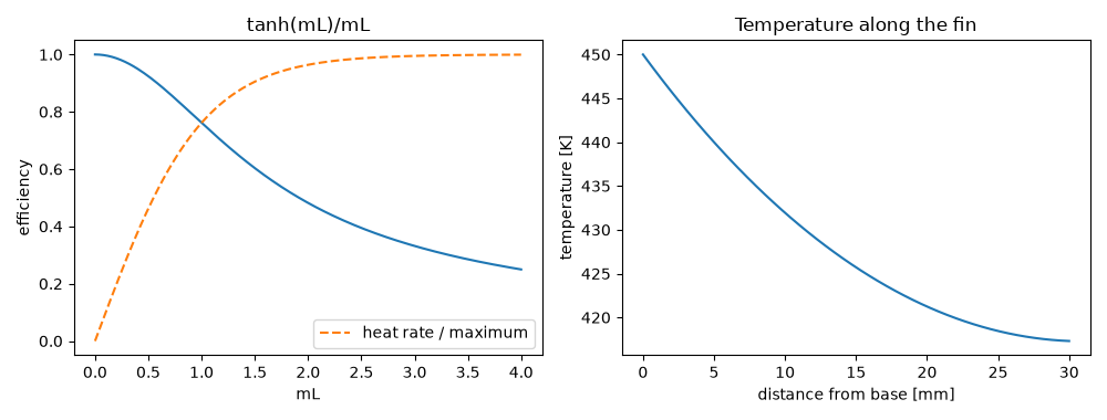
Beyond \(mL \approx 2\) extra length adds almost nothing: the far end of the fin is already at the air temperature.

mL = np.linspace(0, 4, 200)
fig, axes = plt.subplots(1, 2, figsize=(10, 3.8))
axes[0].plot(mL, fin_efficiency_adiabatic(mL, 1.0))
axes[0].plot(mL, np.tanh(mL), "--", label="heat rate / maximum")
axes[0].set(xlabel="mL", ylabel="efficiency", title="tanh(mL)/mL")
axes[0].legend()
axes[1].plot(x * 1e3, Tinf + sol.sol(x)[0])
axes[1].set(xlabel="distance from base [mm]", ylabel="temperature [K]", title="Temperature along the fin")
fig.tight_layout()

plt.show()