Crank and Nicolson: numerical conduction (1947)

In 1947 John Crank and Phyllis Nicolson, solving heat-conduction problems with heat generation on desk calculators, needed a finite-difference scheme for the heat equation that was both stable and accurate. The explicit scheme is stable only for a mesh Fourier number \(r = \alpha\Delta t/\Delta x^2 \le 1/2\); the fully implicit one is always stable but only first order in time. Averaging the two, they got an unconditionally stable, second-order method (conduction_1d()). This example measures the order of each scheme and watches the explicit one blow up.

import matplotlib.pyplot as plt
import numpy as np

from engineeringkit.heat_transfer import conduction_1d

A decaying sine mode

A 100 mm slab with faces held at 300 K starts with a sine-shaped hump. On the grid this mode decays exactly as \(e^{\alpha\lambda t}\) with the discrete eigenvalue \(\lambda = -(4/\Delta x^2)\sin^2(\pi\Delta x/2L)\), so any remaining error comes from the time stepping alone.

L, alpha, n, t_end = 0.1, 1e-5, 51, 200.0
x = np.linspace(0, L, n)
dx = x[1]
T0 = 300.0 + 100.0 * np.sin(np.pi * x / L)
lam = -4 / dx**2 * np.sin(np.pi * dx / (2 * L)) ** 2
reference = 300.0 + 100.0 * np.sin(np.pi * x / L) * np.exp(alpha * lam * t_end)


def error(method, dt):
    result = conduction_1d(T0, L, alpha, dt, round(t_end / dt), T_left=300.0, T_right=300.0, method=method)
    return np.max(np.abs(result.T[-1] - reference)), result.mesh_fourier

Order of accuracy

Halving the time step halves the implicit error and quarters the Crank-Nicolson error, even at mesh Fourier numbers of 20 where the explicit scheme cannot run at all.

steps = [8.0, 4.0, 2.0, 1.0]
fig, axes = plt.subplots(1, 2, figsize=(10, 3.8))
for method in ["implicit", "crank_nicolson"]:
    errors = np.array([error(method, dt)[0] for dt in steps])
    orders = np.log2(errors[:-1] / errors[1:])
    print(f"{method:15s}: errors {np.array2string(errors, precision=5)}, observed order {orders.mean():.3f}")
    assert np.allclose(orders, 1.0 if method == "implicit" else 2.0, atol=0.02)
    axes[0].loglog(steps, errors, "o-", label=method)
explicit_error, r = error("explicit", 0.2)
print(f"explicit at r = {r:.2f}: error {explicit_error:.5f}")
axes[0].loglog([0.2], [explicit_error], "s", label=f"explicit, r = {r:.2f}")
axes[0].set(xlabel="time step [s]", ylabel="max error [K]", title="Convergence in time")
axes[0].legend()

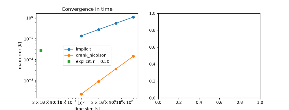
implicit       : errors [1.06772 0.53755 0.2697  0.13508], observed order 0.994
crank_nicolson : errors [0.01425 0.00356 0.00089 0.00022], observed order 2.000
explicit at r = 0.50: error 0.02707

<matplotlib.legend.Legend object at 0x10f802350>

The explicit instability

Above \(r = 1/2\) the explicit scheme amplifies the shortest wave on the grid by \(|1 - 4r|\) per step. Round-off seeds it, and within about a hundred steps a checkerboard swamps the solution. Crank-Nicolson with the same step is unaffected.

dt = 0.6 * dx**2 / alpha
explicit = conduction_1d(T0, L, alpha, dt, 110, T_left=300.0, T_right=300.0, method="explicit")
crank = conduction_1d(T0, L, alpha, dt, 110, T_left=300.0, T_right=300.0)
exact = 300.0 + 100.0 * np.sin(np.pi * x / L) * np.exp(alpha * lam * 110 * dt)
print(
    f"r = {explicit.mesh_fourier:.2f}: explicit error {np.max(np.abs(explicit.T[-1] - exact)):.3g} K, "
    f"Crank-Nicolson error {np.max(np.abs(crank.T[-1] - exact)):.2g} K"
)
assert np.max(np.abs(explicit.T[-1] - exact)) > 1.0 > 1e3 * np.max(np.abs(crank.T[-1] - exact))
axes[1].plot(x * 1e3, explicit.T[-1], label="explicit")
axes[1].plot(x * 1e3, crank.T[-1], label="Crank-Nicolson")
axes[1].set(xlabel="position [mm]", ylabel="temperature [K]", title=f"After 110 steps at r = {explicit.mesh_fourier:.1f}")
axes[1].legend()
fig.tight_layout()

plt.show()

r = 0.60: explicit error 70.9 K, Crank-Nicolson error 9.4e-06 K