Newton’s law of cooling (1701)

In 1701 Newton published, anonymously, a temperature scale reaching far beyond the melting point of tin. He heated a block of iron red hot, set it in a steady wind, and timed how long it took to cool. Assuming that the heat lost is proportional to the excess temperature, \(\dot Q = hA(T - T_\infty)\) (convection_heat_rate()), equal intervals of time should multiply the excess temperature by equal factors (lumped_temperature()). Newton then read temperatures off the clock. This example repeats the measurement on a model block, recovers the time constant from the readings, and checks the energy balance.

import matplotlib.pyplot as plt
import numpy as np
from scipy import integrate

from engineeringkit.heat_transfer import convection_heat_rate, lumped_temperature

Equal times, equal ratios

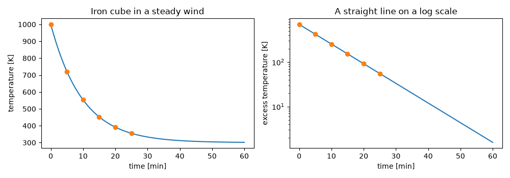
A 4 cm iron cube (\(\rho = 7870\) kg/m³, \(c_p = 450\) J/(kg K)) cools from 1000 K in a 300 K wind with \(h = 40\) W/(m² K).

rho, cp, side, h, Ti, Tinf = 7870.0, 450.0, 0.04, 40.0, 1000.0, 300.0
A, V = 6 * side**2, side**3
tau = rho * cp * V / (h * A)
readings = np.arange(0, 6) * 300.0  # every five minutes
excess = lumped_temperature(Ti, Tinf, h, A, rho, cp, V, readings) - Tinf
ratios = excess[1:] / excess[:-1]
print(f"time constant {tau:.0f} s")
print("excess temperature [K]:", np.round(excess, 1))
print("ratio between readings:", np.round(ratios, 4))
assert np.allclose(ratios, np.exp(-300.0 / tau))

time constant 590 s
excess temperature [K]: [700.  421.1 253.3 152.4  91.7  55.1]
ratio between readings: [0.6015 0.6015 0.6015 0.6015 0.6015]

Reading temperature off the clock

The slope of \(\ln(T - T_\infty)\) against time is \(-1/\tau\), so the readings alone give the time constant, and from it the temperature at any earlier time, which is how Newton reached beyond his linseed-oil thermometer.

slope, intercept = np.polyfit(readings, np.log(excess), 1)
print(f"fitted time constant {-1 / slope:.0f} s, back-extrapolated start {Tinf + np.exp(intercept):.1f} K")
assert np.isclose(-1 / slope, tau) and np.isclose(Tinf + np.exp(intercept), Ti)

fitted time constant 590 s, back-extrapolated start 1000.0 K

Energy balance

The heat convected away over the first hour equals the drop in the block’s stored energy.

t = np.linspace(0, 3600, 3601)
T = lumped_temperature(Ti, Tinf, h, A, rho, cp, V, t)
lost = integrate.trapezoid(convection_heat_rate(h, A, T, Tinf), t)
stored = rho * cp * V * (Ti - T[-1])
print(f"heat convected {lost / 1e3:.2f} kJ, stored energy released {stored / 1e3:.2f} kJ")
assert np.isclose(lost, stored, rtol=1e-6)

fig, axes = plt.subplots(1, 2, figsize=(10, 3.5))
axes[0].plot(t / 60, T)
axes[0].plot(readings / 60, Tinf + excess, "o")
axes[0].set(xlabel="time [min]", ylabel="temperature [K]", title="Iron cube in a steady wind")
axes[1].semilogy(t / 60, T - Tinf)
axes[1].semilogy(readings / 60, excess, "o")
axes[1].set(xlabel="time [min]", ylabel="excess temperature [K]", title="A straight line on a log scale")
fig.tight_layout()

plt.show()

heat convected 158.30 kJ, stored energy released 158.30 kJ