Churchill and Chu: natural convection over all Rayleigh numbers (1975)

Free convection on a vertical plate was long described piecewise: a laminar \(Ra^{1/4}\) law, a turbulent \(Ra^{1/3}\) law, and a gap between them. In 1975 Stuart Churchill and Humbert Chu fitted one smooth expression to the data from conduction-dominated creeping flow to fully turbulent plumes, \(Nu = \{0.825 + 0.387 Ra^{1/6}/[1 + (0.492/Pr)^{9/16}]^{8/27}\}^2\) (churchill_chu_nusselt(), with rayleigh_number()). The example checks both asymptotes and the laminar boundary-layer theory it replaces.

import matplotlib.pyplot as plt
import numpy as np

from engineeringkit.heat_transfer import churchill_chu_nusselt, rayleigh_number

A warm wall in still air

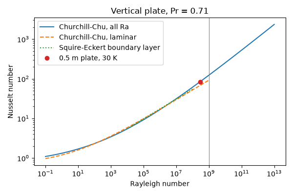
A 0.5 m tall plate at 330 K in air at 300 K; properties at the 315 K film temperature.

beta, nu, alpha, k, Pr, H = 1 / 315.0, 1.70e-5, 2.40e-5, 0.0274, 0.71, 0.5
Ra = rayleigh_number(beta, 30.0, H, nu, alpha)
Nu = churchill_chu_nusselt(Ra, Pr)
print(f"Ra = {Ra:.3e}, Nu = {Nu:.1f}, h = {Nu * k / H:.2f} W/(m² K)")

Ra = 2.861e+08, Nu = 83.8, h = 4.59 W/(m² K)

Laminar range: the boundary-layer solution

The Squire-Eckert integral solution of the laminar boundary layer gives \(Nu = 0.678\,Ra^{1/4}[Pr/(0.952 + Pr)]^{1/4}\). Below \(Ra = 10^9\) it agrees with Churchill and Chu’s laminar form and their all-range form.

Ra_lam = np.geomspace(1e4, 1e8, 30)
squire_eckert = 0.678 * Ra_lam**0.25 * (Pr / (0.952 + Pr)) ** 0.25
lam_gap = np.max(np.abs(churchill_chu_nusselt(Ra_lam, Pr, laminar=True) / squire_eckert - 1))
all_gap = np.max(np.abs(churchill_chu_nusselt(Ra_lam, Pr) / squire_eckert - 1))
print(f"vs Squire-Eckert: laminar form within {lam_gap:.1%}, all-range form within {all_gap:.1%}")
assert lam_gap < 0.07 and all_gap < 0.12

vs Squire-Eckert: laminar form within 6.2%, all-range form within 11.4%

Turbulent range: the one-third law

In turbulent free convection the heat flux no longer depends on the plate height, which requires \(Nu \propto Ra^{1/3}\).

slope = np.log(churchill_chu_nusselt(1e14, Pr) / churchill_chu_nusselt(1e13, Pr)) / np.log(10)
print(f"log-log slope between Ra = 1e13 and 1e14: {slope:.3f}")
assert abs(slope - 1 / 3) < 0.01

Ra_all = np.geomspace(1e-1, 1e13, 200)
fig, ax = plt.subplots(figsize=(6, 4))
ax.loglog(Ra_all, churchill_chu_nusselt(Ra_all, Pr), label="Churchill-Chu, all Ra")
ax.loglog(Ra_all[Ra_all < 1e9], churchill_chu_nusselt(Ra_all[Ra_all < 1e9], Pr, laminar=True), "--", label="Churchill-Chu, laminar")
ax.loglog(Ra_lam, squire_eckert, ":", label="Squire-Eckert boundary layer")
ax.axvline(1e9, color="gray", lw=0.8)
ax.plot(Ra, Nu, "o", label="0.5 m plate, 30 K")
ax.set(xlabel="Rayleigh number", ylabel="Nusselt number", title="Vertical plate, Pr = 0.71")
ax.legend()
fig.tight_layout()

plt.show()

log-log slope between Ra = 1e13 and 1e14: 0.329