Pohlhausen’s thermal boundary layer (1921)

Blasius (1908) had reduced Prandtl’s laminar boundary layer on a flat plate to one ordinary differential equation, \(f''' + \tfrac12 ff'' = 0\). In 1921 Ernst Pohlhausen, also in Prandtl’s Göttingen, added the energy equation. With the same similarity variable it becomes \(\theta'' + \tfrac12 Pr\,f\theta' = 0\), which integrates in closed form once \(f\) is known, and the wall gradient is close to \(0.332\,Pr^{1/3}\) for every Prandtl number of gases and ordinary liquids. That gives \(Nu_x = 0.332\,Re_x^{1/2}Pr^{1/3}\), the starting point of every convection course (flat_plate_nusselt()). This example solves Blasius and Pohlhausen’s equations and then cools a plate whose boundary layer turns turbulent.

import matplotlib.pyplot as plt
import numpy as np
from scipy.integrate import cumulative_trapezoid, solve_ivp, trapezoid
from scipy.optimize import brentq

from engineeringkit.heat_transfer import flat_plate_nusselt

Blasius’s velocity profile

Shoot on the unknown wall curvature \(f''(0)\) until \(f' \to 1\) far from the wall.

eta = np.linspace(0, 12, 12001)


def blasius(curvature):
    return solve_ivp(lambda e, y: [y[1], y[2], -0.5 * y[0] * y[2]], [0, 12], [0, 0, curvature], t_eval=eta, rtol=1e-11, atol=1e-12)


curvature = brentq(lambda c: blasius(c).y[1, -1] - 1, 0.2, 0.5, xtol=1e-12)
f = blasius(curvature).y[0]
print(f"f''(0) = {curvature:.5f}")
assert abs(curvature - 0.33206) < 1e-5

f''(0) = 0.33206

Pohlhausen’s temperature profile

\(\theta'' = -\tfrac12 Pr f\theta'\) gives \(\theta'(\eta) = \theta'(0)\exp(-\tfrac12 Pr\int_0^\eta f)\), and \(\theta(\infty) = 1\) fixes \(\theta'(0)\).

F = cumulative_trapezoid(f, eta, initial=0)
Prs = np.geomspace(0.6, 100, 25)
gradient = np.array([1 / trapezoid(np.exp(-Pr / 2 * F), eta) for Pr in Prs])
fit = flat_plate_nusselt(1.0, Prs, local=True)  # 0.332 Pr^(1/3) at Re_x = 1
worst = np.max(np.abs(fit / gradient - 1))
print(f"0.332 Pr^(1/3) against the exact wall gradient for 0.6 < Pr < 100: within {worst:.1%}")
assert worst < 0.025

fig, axes = plt.subplots(1, 2, figsize=(10, 3.8))
axes[0].plot(blasius(curvature).y[1], eta, label="velocity f'")
for Pr in [0.7, 7.0, 70.0]:
    theta = cumulative_trapezoid(np.exp(-Pr / 2 * F), eta, initial=0) / trapezoid(np.exp(-Pr / 2 * F), eta)
    axes[0].plot(theta, eta, "--", label=f"temperature, Pr = {Pr:g}")
axes[0].set(xlabel="u/U, (T - Ts)/(T∞ - Ts)", ylabel="η = y (U/νx)^1/2", ylim=(0, 8), title="Similarity profiles")
axes[0].legend()
axes[1].loglog(Prs, gradient, "o", label="exact θ'(0)")
axes[1].loglog(Prs, fit, label="0.332 Pr^1/3")
axes[1].set(xlabel="Prandtl number", ylabel="θ'(0) = Nu_x / Re_x^1/2", title="Pohlhausen's result")
axes[1].legend()
fig.tight_layout()

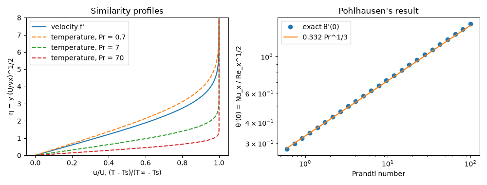
0.332 Pr^(1/3) against the exact wall gradient for 0.6 < Pr < 100: within 2.0%

A plate that turns turbulent

Air at 300 K and 10 m/s over a 1.5 m plate: transition at \(Re = 5\times10^5\) (0.75 m). The local coefficient jumps where the boundary layer turns turbulent, and the average follows from integrating it.

nu, k, Pr, U, L = 1.589e-5, 0.0263, 0.707, 10.0, 1.5
x = np.linspace(1e-4, L, 4000)
h_local = flat_plate_nusselt(U * x / nu, Pr, local=True) * k / x
h_mean = flat_plate_nusselt(U * L / nu, Pr) * k / L
h_integrated = trapezoid(h_local, x) / L
print(f"Re_L = {U * L / nu:.3g}: mean h = {h_mean:.2f} W/(m² K), integrated local h = {h_integrated:.2f}")
assert abs(h_integrated / h_mean - 1) < 0.01

fig, ax = plt.subplots(figsize=(6, 3.5))
ax.plot(x, h_local)
ax.axhline(h_mean, color="gray", ls="--", label=f"mean {h_mean:.1f} W/(m² K)")
ax.set(xlabel="distance from leading edge [m]", ylabel="local h [W/(m² K)]", ylim=(0, 40), title="Mixed boundary layer")
ax.legend()
fig.tight_layout()

plt.show()

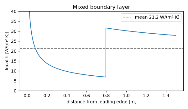
Re_L = 9.44e+05: mean h = 21.21 W/(m² K), integrated local h = 21.14