The Chilton-Colburn analogy (1934)

Allan Colburn at DuPont noticed in 1933 that turbulent heat transfer data collapse when the Stanton number is multiplied by \(Pr^{2/3}\), and that this \(j\) factor equals half the friction factor. In 1934, with Thomas Chilton, he carried the same factor over to mass transfer: if \(St\,Pr^{2/3} = St_m Sc^{2/3}\), a heat transfer coefficient gives the mass transfer coefficient, \(h_m = h/(\rho c_p Le^{2/3})\) (chilton_colburn_mass_transfer()). It lets one experiment stand for three. This example checks the analogy on the laminar flat plate and uses it to explain the wet-bulb thermometer.

import matplotlib.pyplot as plt
import numpy as np
from scipy.optimize import brentq

from engineeringkit.heat_transfer import chilton_colburn_mass_transfer, flat_plate_nusselt, lewis_number

The flat plate: heat, mass and momentum

On the laminar flat plate \(Nu = 0.664 Re^{1/2}Pr^{1/3}\), the concentration boundary layer obeys the same equation with \(Sc\) for \(Pr\), and the friction coefficient is \(C_f = 1.328 Re^{-1/2}\). All three \(j\) factors agree.

Re, Pr, Sc = 2e5, 0.71, 0.60
j_heat = flat_plate_nusselt(Re, Pr) / (Re * Pr) * Pr ** (2 / 3)
j_mass = flat_plate_nusselt(Re, Sc) / (Re * Sc) * Sc ** (2 / 3)
half_cf = 0.5 * 1.328 / np.sqrt(Re)
print(f"j_H = {j_heat:.6f}, j_m = {j_mass:.6f}, Cf/2 = {half_cf:.6f}")
assert np.isclose(j_heat, j_mass) and np.isclose(j_heat, half_cf)

j_H = 0.001485, j_m = 0.001485, Cf/2 = 0.001485

The wet-bulb thermometer

A wetted wick in moving air cools until the heat convected to it equals the latent heat carried off by evaporation: \(h(T_\infty - T_{wb}) = h_m h_{fg}[\rho_{v,sat}(T_{wb}) - \rho_{v,\infty}]\). The analogy makes \(h/h_m = \rho c_p Le^{2/3}\), so the reading does not depend on the air speed. Air at 30 °C and 40% relative humidity:

rho, cp, h_fg, R_v = 1.16, 1007.0, 2.43e6, 461.5
Le = lewis_number(2.25e-5, 2.6e-5)


def p_sat(T):
    """Saturation pressure of water [Pa] (Magnus formula, T in K)."""
    return 610.94 * np.exp(17.625 * (T - 273.15) / (T - 30.11))


T_air, rh = 303.15, 0.40
rho_v_air = rh * p_sat(T_air) / (R_v * T_air)
for h in [10.0, 40.0, 160.0]:
    h_m = chilton_colburn_mass_transfer(h, rho, cp, Le)
    T_wb = brentq(lambda T: h * (T_air - T) - h_m * h_fg * (p_sat(T) / (R_v * T) - rho_v_air), 273.2, T_air)
    print(f"h = {h:5.0f} W/(m² K): h_m = {h_m * 1000:.2f} mm/s, wet bulb {T_wb - 273.15:.2f} °C")
print(f"Lewis number {Le:.3f}; psychrometric tables give about 20.0 °C for these conditions")
assert abs(T_wb - 273.15 - 20.0) < 0.6

speeds = np.geomspace(1, 300, 50)
wet = [
    brentq(
        lambda T, h=h: h * (T_air - T) - chilton_colburn_mass_transfer(h, rho, cp, Le) * h_fg * (p_sat(T) / (R_v * T) - rho_v_air),
        273.2,
        T_air,
    )
    for h in speeds
]
fig, ax = plt.subplots(figsize=(6, 3.5))
ax.semilogx(speeds, np.array(wet) - 273.15)
ax.set(
    xlabel="convection coefficient [W/(m² K)]",
    ylabel="wet-bulb temperature [°C]",
    ylim=(15, 25),
    title="The analogy makes the wet bulb speed-independent",
)
fig.tight_layout()

plt.show()

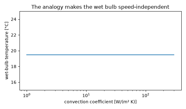
h =    10 W/(m² K): h_m = 9.43 mm/s, wet bulb 19.46 °C
h =    40 W/(m² K): h_m = 37.71 mm/s, wet bulb 19.46 °C
h =   160 W/(m² K): h_m = 150.83 mm/s, wet bulb 19.46 °C
Lewis number 0.865; psychrometric tables give about 20.0 °C for these conditions