Kirchhoff’s law of thermal radiation (1859)

In 1859 Gustav Kirchhoff, explaining the dark lines that Fraunhofer had seen in the solar spectrum, proved from the second law that at every wavelength a body’s emissivity equals its absorptivity. A good absorber is a good emitter, and the perfect absorber, the blackbody, is the universal reference whose emission depends on temperature alone. For a gray surface in large surroundings the net exchange is \(\varepsilon\sigma A(T_s^4 - T_{sur}^4)\) (radiation_heat_rate()), often linearised as a coefficient \(h_r\) (radiation_coefficient()). This example shows why \(\alpha = \varepsilon\) is forced: anything else would let heat flow from cold to hot.

import matplotlib.pyplot as plt
import numpy as np
from scipy.integrate import solve_ivp

from engineeringkit.heat_transfer import STEFAN_BOLTZMANN, convection_heat_rate, radiation_coefficient, radiation_heat_rate

A body in an isothermal enclosure

A small plate of area \(A\) absorbs \(\alpha\sigma T_{sur}^4 A\) and emits \(\varepsilon\sigma T^4 A\). Integrate its temperature for Kirchhoff’s \(\alpha = \varepsilon\) and for a hypothetical surface with \(\alpha = 0.9\), \(\varepsilon = 0.3\).

A, m_cp, T_sur = 0.01, 5.0, 500.0


def net_gain(alpha, epsilon):
    return lambda t, T: [(alpha * T_sur**4 - epsilon * T[0] ** 4) * STEFAN_BOLTZMANN * A / m_cp]


t_end = 1800.0
fig, axes = plt.subplots(1, 2, figsize=(10, 3.8))
finals = {}
for label, (a, e) in {"α = ε = 0.9": (0.9, 0.9), "α = ε = 0.3": (0.3, 0.3), "α = 0.9, ε = 0.3": (0.9, 0.3)}.items():
    sol = solve_ivp(net_gain(a, e), (0, t_end), [300.0], rtol=1e-10, atol=1e-8, dense_output=True)
    finals[label] = sol.y[0, -1]
    t = np.linspace(0, t_end, 300)
    axes[0].plot(t / 60, sol.sol(t)[0], label=label)
    print(f"{label:17s}: final temperature {finals[label]:.1f} K")
axes[0].axhline(T_sur, color="k", ls=":")
axes[0].set(xlabel="time [min]", ylabel="plate temperature [K]", title="Plate in a 500 K enclosure")
axes[0].legend()

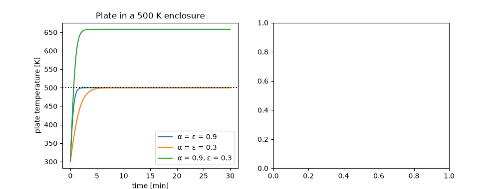
α = ε = 0.9      : final temperature 500.0 K
α = ε = 0.3      : final temperature 500.0 K
α = 0.9, ε = 0.3 : final temperature 658.0 K

<matplotlib.legend.Legend object at 0x111257390>

With \(\alpha = \varepsilon\) every plate settles at the enclosure temperature, as the second law demands. The hypothetical surface would heat itself to \((\alpha/\varepsilon)^{1/4}T_{sur}\), above its surroundings: a perpetual motion of the second kind.

assert np.isclose(finals["α = ε = 0.9"], T_sur, rtol=1e-6) and np.isclose(finals["α = ε = 0.3"], T_sur, rtol=1e-6)
assert np.isclose(finals["α = 0.9, ε = 0.3"], 3**0.25 * T_sur, rtol=1e-6)
for e in [0.1, 0.5, 1.0]:
    assert radiation_heat_rate(e, A, T_sur, T_sur) == 0.0

Radiation as a heat-transfer coefficient

\(h_r = \varepsilon\sigma(T_s + T_{sur})(T_s^2 + T_{sur}^2)\) makes radiation exact in convection form, and it grows fast with temperature: at furnace temperatures it dwarfs natural convection.

Ts = np.linspace(310, 1300, 100)
hr = radiation_coefficient(0.8, Ts, 300.0)
assert np.allclose(hr * A * (Ts - 300.0), radiation_heat_rate(0.8, A, Ts, 300.0))
assert np.allclose(convection_heat_rate(hr, A, Ts, 300.0), radiation_heat_rate(0.8, A, Ts, 300.0))
print(f"h_r for ε = 0.8 against 300 K: {hr[0]:.1f} W/(m² K) at 310 K, {hr[-1]:.0f} W/(m² K) at 1300 K")
axes[1].plot(Ts, hr, label="radiation, ε = 0.8")
axes[1].axhline(5.0, color="C1", ls="--", label="typical natural convection")
axes[1].set(xlabel="surface temperature [K]", ylabel="coefficient [W/(m² K)]", title="Linearised radiation")
axes[1].legend()
fig.tight_layout()

plt.show()

h_r for ε = 0.8 against 300 K: 5.1 W/(m² K) at 310 K, 129 W/(m² K) at 1300 K