Stefan and Boltzmann: emission grows as T⁴ (1879-1884)

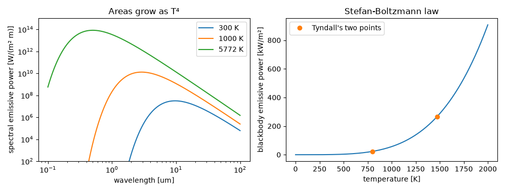
In 1879 Josef Stefan reread John Tyndall’s measurements of a glowing platinum wire: at 1200 °C it radiated 11.7 times as much as at 525 °C. The ratio of the absolute temperatures to the fourth power is 11.6, and Stefan proposed \(E \propto T^4\). In 1884 his former student Ludwig Boltzmann derived the law from thermodynamics and Maxwell’s radiation pressure, \(E_b = \sigma T^4\) (stefan_boltzmann_emissive_power()). The constant \(\sigma\) was explained only by Planck’s spectrum (planck_spectral_emissive_power()), whose integral this example checks against the law.

import matplotlib.pyplot as plt
import numpy as np
from scipy import integrate

from engineeringkit.heat_transfer import STEFAN_BOLTZMANN, planck_spectral_emissive_power, stefan_boltzmann_emissive_power
from engineeringkit.heat_transfer.utils import BOLTZMANN, PLANCK, SPEED_OF_LIGHT

Tyndall’s platinum wire

T_hot, T_cold = 1200 + 273.0, 525 + 273.0
ratio = stefan_boltzmann_emissive_power(T_hot) / stefan_boltzmann_emissive_power(T_cold)
print(f"(T_hot/T_cold)^4 = {ratio:.2f}, Tyndall measured 11.7")
assert abs(ratio - 11.7) < 0.2

(T_hot/T_cold)^4 = 11.61, Tyndall measured 11.7

The constant from the spectrum

Integrating Planck’s law over all wavelengths gives \(\sigma = 2\pi^5k^4/(15h^3c^2)\).

sigma_theory = 2 * np.pi**5 * BOLTZMANN**4 / (15 * PLANCK**3 * SPEED_OF_LIGHT**2)
print(f"sigma from h, c, k: {sigma_theory:.6e} W/(m² K⁴); CODATA {STEFAN_BOLTZMANN:.6e}")
assert np.isclose(sigma_theory, STEFAN_BOLTZMANN, rtol=1e-9)

fig, axes = plt.subplots(1, 2, figsize=(10, 3.8))
for T in [300.0, 1000.0, 5772.0]:
    total, _ = integrate.quad(planck_spectral_emissive_power, 1e-9, 1e-2, args=(T,), points=[2.9e-3 / T], limit=200)
    print(f"T = {T:6.0f} K: integral of Planck {total:.6e} W/m², sigma T^4 {stefan_boltzmann_emissive_power(T):.6e} W/m²")
    assert np.isclose(total, stefan_boltzmann_emissive_power(T), rtol=1e-5)
    lam = np.geomspace(0.1e-6, 100e-6, 500)
    axes[0].loglog(lam * 1e6, planck_spectral_emissive_power(lam, T), label=f"{T:.0f} K")
axes[0].set(xlabel="wavelength [um]", ylabel="spectral emissive power [W/(m² m)]", ylim=(1e2, 1e15), title="Areas grow as T⁴")
axes[0].legend()

T = np.linspace(0, 2000, 200)
axes[1].plot(T, stefan_boltzmann_emissive_power(T) / 1e3)
axes[1].plot([T_cold, T_hot], stefan_boltzmann_emissive_power(np.array([T_cold, T_hot])) / 1e3, "o", label="Tyndall's two points")
axes[1].set(xlabel="temperature [K]", ylabel="blackbody emissive power [kW/m²]", title="Stefan-Boltzmann law")
axes[1].legend()
fig.tight_layout()

plt.show()

sigma from h, c, k: 5.670374e-08 W/(m² K⁴); CODATA 5.670374e-08
T =    300 K: integral of Planck 4.593003e+02 W/m², sigma T^4 4.593003e+02 W/m²
T =   1000 K: integral of Planck 5.670374e+04 W/m², sigma T^4 5.670374e+04 W/m²
T =   5772 K: integral of Planck 6.293859e+07 W/m², sigma T^4 6.293859e+07 W/m²