Wien’s displacement law (1893)

In 1893 Wilhelm Wien imagined blackbody radiation compressed adiabatically in a cavity with a moving mirror. Doppler shifts and the second law then forced the spectrum to keep its shape as the temperature changes: the spectral emissive power divided by \(T^5\) depends only on \(\lambda T\). Its peak therefore sits at \(\lambda_{max}T = b\) (blackbody_peak_wavelength()), with \(b = 2898\) um K. The law says why the Sun peaks in the visible, a lamp filament in the near infrared and a person at about 10 um. This example finds the peak of Planck’s spectrum numerically and checks the similarity that Wien proved.

import matplotlib.pyplot as plt
import numpy as np
from scipy.optimize import minimize_scalar

from engineeringkit.heat_transfer import WIEN_DISPLACEMENT, blackbody_peak_wavelength, planck_spectral_emissive_power
from engineeringkit.heat_transfer.visualizers import plot_blackbody_spectra

The peak of Planck’s curve

sources = {"human skin": 305.0, "red-hot iron": 1000.0, "tungsten filament": 2800.0, "Sun's photosphere": 5772.0}
for name, T in sources.items():
    guess = 2898 / T  # um
    peak = minimize_scalar(lambda lam_um: -planck_spectral_emissive_power(lam_um * 1e-6, T), bracket=(0.5 * guess, guess, 2 * guess)).x
    print(f"{name:18s} {T:6.0f} K: numerical peak {peak:7.3f} um, b/T {blackbody_peak_wavelength(T) * 1e6:7.3f} um")
    assert np.isclose(peak * 1e-6, blackbody_peak_wavelength(T), rtol=1e-5)

human skin            305 K: numerical peak   9.501 um, b/T   9.501 um
red-hot iron         1000 K: numerical peak   2.898 um, b/T   2.898 um
tungsten filament    2800 K: numerical peak   1.035 um, b/T   1.035 um
Sun's photosphere    5772 K: numerical peak   0.502 um, b/T   0.502 um

One curve for every temperature

Plotted as \(E_{\lambda,b}/T^5\) against \(\lambda T\), all the spectra collapse onto one curve, whose maximum is at \(b\).

lamT = np.geomspace(500e-6, 50000e-6, 400)
collapsed = [planck_spectral_emissive_power(lamT / T, T) / T**5 for T in sources.values()]
assert np.allclose(collapsed, collapsed[0], rtol=1e-12)
peak_lamT = lamT[np.argmax(collapsed[0])] * 1e6
print(f"all four spectra coincide when scaled; peak at lambda T = {peak_lamT:.0f} um K (b = {WIEN_DISPLACEMENT * 1e6:.1f})")

fig, axes = plt.subplots(1, 2, figsize=(10, 3.8))
plot_blackbody_spectra(list(sources.values()), ax=axes[0])
axes[0].set_ylim(1e3, 1e14)
axes[0].axvspan(0.38, 0.75, color="gold", alpha=0.3)
axes[0].set_title("Peaks move to shorter wavelengths")
axes[1].semilogx(lamT * 1e6, collapsed[0])
axes[1].axvline(WIEN_DISPLACEMENT * 1e6, color="k", ls=":")
axes[1].set(xlabel="λT [um K]", ylabel="E / T⁵ [W/(m³ K⁵)]", title="Wien's similarity")
fig.tight_layout()

plt.show()

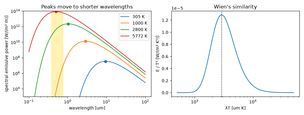
all four spectra coincide when scaled; peak at lambda T = 2890 um K (b = 2897.8)