Biot’s heated bar and the Biot number (1804)

In 1804 Jean-Baptiste Biot heated one end of iron bars and read thermometers set along them. He saw that the temperature profile is set by a contest between conduction along the bar and loss from its surface. He could not write a consistent differential equation for it; Fourier did in 1807. The ratio of the two effects, now the Biot number \(Bi = hL/k\) (biot_number()), decides whether a body can be treated as a single temperature. This example cools a plane wall at three Biot numbers and compares the lumped model \(e^{-Bi\,Fo}\) with the exact series solution.

import matplotlib.pyplot as plt
import numpy as np
from scipy import integrate

from engineeringkit.heat_transfer import biot_number, fourier_number, plane_wall_transient

The same wall, three coolants

A 40 mm steel plate (\(k = 40\) W/(m K), half-thickness \(L = 20\) mm) cooled on both faces by still air, forced air and a water spray.

k, L = 40.0, 0.02
coolants = {"still air": 20.0, "air jet": 200.0, "water spray": 2000.0}
Bis = {name: biot_number(h, L, k) for name, h in coolants.items()}
for name, Bi in Bis.items():
    print(f"{name:12s}: Bi = {Bi:.2f}")

still air   : Bi = 0.01
air jet     : Bi = 0.10
water spray : Bi = 1.00

Lumped versus distributed

A lumped body follows \(\theta = e^{-Bi\,Fo}\). The exact mean temperature of the wall averages the series over the thickness.

x_star = np.linspace(0, 1, 201)
Fo = np.linspace(0, 3, 61)[1:]
fig, axes = plt.subplots(1, 2, figsize=(10, 3.8))
for name, Bi in Bis.items():
    mean = np.array([integrate.trapezoid(plane_wall_transient(F, Bi, x_star), x_star) for F in Fo])
    lumped = np.exp(-Bi * Fo)
    error = np.max(np.abs(lumped - mean))
    print(f"{name:12s}: worst lumped error {error:.4f} (fraction of the initial excess)")
    line = axes[0].plot(Fo, mean, label=f"exact, Bi = {Bi:.2f}")[0]
    axes[0].plot(Fo, lumped, "--", color=line.get_color())
    axes[1].plot(x_star, plane_wall_transient(0.5, Bi, x_star), color=line.get_color(), label=f"Bi = {Bi:.2f}")
    if Bi <= 0.1:
        assert error < 0.01
    else:
        assert error > 0.1
axes[0].set(xlabel="Fourier number", ylabel="mean excess temperature", title="Solid: exact, dashed: lumped")
axes[0].legend()
axes[1].set(xlabel="x / L (centre to surface)", ylabel="excess temperature", title="Profiles at Fo = 0.5")
axes[1].legend()
fig.tight_layout()

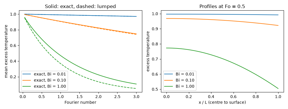
still air   : worst lumped error 0.0001 (fraction of the initial excess)
air jet     : worst lumped error 0.0071 (fraction of the initial excess)
water spray : worst lumped error 0.1045 (fraction of the initial excess)

What the time scale means

In the still-air case the plate is effectively isothermal, and an hour of cooling is \(Fo\) of order 100 on the half-thickness.

alpha = k / (7850.0 * 460.0)
print(f"one hour is Fo = {fourier_number(alpha, 3600.0, L):.0f}")

plt.show()

one hour is Fo = 100