Yule’s autoregressive model (1927)

Schuster’s periodogram looked for strict periodicities hidden in noise. George Udny Yule, studying Wolfer’s sunspot numbers, proposed another picture: a pendulum “pelted with peas”, a damped oscillator kept going by random shocks, \(x_n = -a_1 x_{n-1} - a_2 x_{n-2} + e_n\). Its cycle wanders in phase and amplitude, as the sunspot cycle does, and it is fitted from the record’s correlations, not its Fourier coefficients. Gilbert Walker (1931) extended the equations to any order. The fitted model gives a smooth spectrum \(\sigma^2/|A(e^{j\omega})|^2\) (yule_walker(), ARModel).

import matplotlib.pyplot as plt
import numpy as np
from scipy import signal

from engineeringkit.signal_processing import power_spectral_density, yule_walker

A disturbed pendulum with an 11-year period

Poles at radius 0.9 and angle \(2\pi/11\) per year give a damped oscillator; white shocks keep it ringing. 300 years of annual values.

radius, period = 0.9, 11.0
a_true = np.array([1.0, -2 * radius * np.cos(2 * np.pi / period), radius**2])
rng = np.random.default_rng(1927)
x = signal.lfilter([1.0], a_true, rng.normal(size=600))[300:] + 50.0
years = 1700 + np.arange(x.size)
fig, axes = plt.subplots(1, 2, figsize=(11, 4))
axes[0].plot(years, x)
axes[0].set(xlabel="year", ylabel="activity", title="Yule's process: no fixed phase or amplitude")

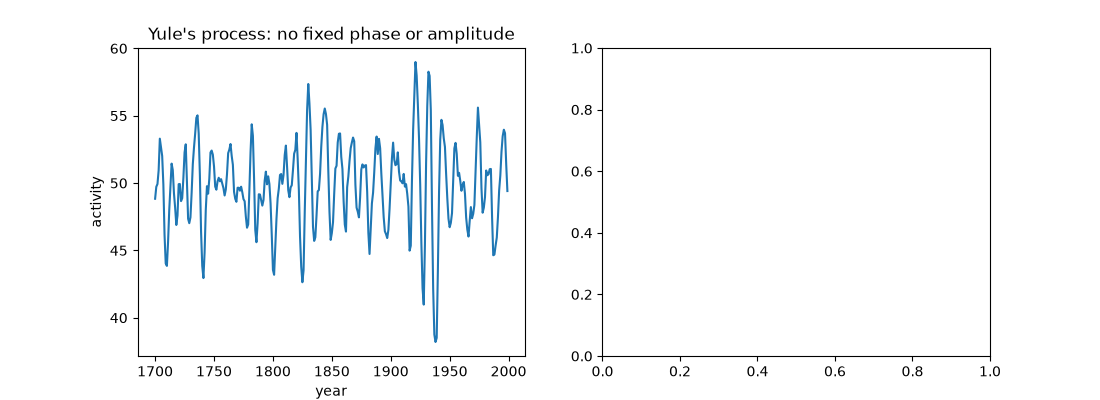
[Text(0.5, 14.833333333333327, 'year'), Text(104.22222222222221, 0.5, 'activity'), Text(0.5, 1.0, "Yule's process: no fixed phase or amplitude")]

Fit by the Yule-Walker equations

model = yule_walker(x, 2)
print("fitted A(z):", np.round(model.coefficients, 3), " true:", np.round(a_true, 3))
print(model.summary())
poles = np.roots(model.coefficients)
fitted_period = 2 * np.pi / np.abs(np.angle(poles[0]))
print(f"pole radius {abs(poles[0]):.3f}, period {fitted_period:.1f} years")

fitted A(z): [ 1.    -1.516  0.812]  true: [ 1.    -1.514  0.81 ]
{'order': 2, 'noise_variance': 1.0905233922949178, 'prediction_gain': 9.765797731115361, 'stable': True}
pole radius 0.901, period 11.0 years

AR spectrum against the periodogram

The periodogram of 300 values is ragged at every frequency; the two-parameter model gives a smooth peak at the same place.

f, P = power_spectral_density(x, 1.0)
f_ar, P_ar = model.psd(fs=1.0, n=1024)
true_psd = 2 / np.abs(np.exp(-2j * np.pi * np.outer(f_ar, np.arange(3))) @ a_true) ** 2
axes[1].semilogy(f[1:], P[1:], color="0.7", lw=0.7, label="periodogram")
axes[1].semilogy(f_ar, P_ar, label="AR(2) fit")
axes[1].semilogy(f_ar, true_psd, "k--", lw=0.8, label="true spectrum")
axes[1].set(xlabel="frequency [1/year]", ylabel="PSD [units²·year]", title="Spectrum")
axes[1].legend()
fig.tight_layout()
peak_period = 1 / f_ar[np.argmax(P_ar)]
print(f"AR spectrum peaks at a period of {peak_period:.1f} years")
assert np.allclose(model.coefficients, a_true, atol=0.06)
assert abs(fitted_period - period) < 1.0 and abs(peak_period - period) < 1.5

plt.show()

AR spectrum peaks at a period of 11.2 years