
Note
Go to the end to download the full example code.
The Position Operator of Wannier Functions in the Anomalous Hall Effect#
A tight-binding model knows the position operator only through its
orbitals. If each orbital sits at its centre and is an eigenstate of
position, \(\mathbf{r}\) is diagonal, the velocity is
\(i[H, \mathbf{r}] = \partial H/\partial\mathbf{k}\) with the centres in
the Bloch phases, and the Berry curvature follows from the bands alone.
Wannier functions computed from first principles are not eigenstates of
position: Wannier90 writes, in seedname_tb.dat, every matrix element
\(\langle m\mathbf{0}|\mathbf{r}|n\mathbf{R}\rangle\), not only the
centres. Wang, Yates, Souza and Vanderbilt (Phys. Rev. B 74, 195118
(2006)) showed how they enter the anomalous Hall conductivity: in the
velocity, \(i[H, \mathbf{r}]\) with the whole operator, and in each
band’s curvature, which gains the curvature of the Wannier functions’ own
Berry connection \(\mathbf{A}(\mathbf{k})\),
Here the same physics is written in two bases. The Haldane model (two
orbitals at their positions) is rewritten in the basis
\(V(\mathbf{k}) = e^{i\epsilon S(\mathbf{k})}\), a k-dependent
unitary mixing of the orbitals, as a Wannierization would produce: its
Hamiltonian is \(V^\dagger HV\), its connection
\(V^\dagger\boldsymbol\tau V + iV^\dagger\nabla_{\mathbf{k}}V\), with
elements off the diagonal and between cells, and centres away from the
atoms. write_tb() writes it as a _tb.dat file, and
read_wannier90_tb() reads it back with its position
matrix elements, or with the centres alone (elements=False).
import os
import tempfile

import numpy as np
import scipy.linalg as sla
import matplotlib.pyplot as plt

from tbkit import models
from tbkit.io import _hr_kspace, read_wannier90_tb, write_tb

hal = models.haldane(t2=0.15, phi=np.pi / 2, M=0.1)


def rotated(ks, eps=0.6, n=25):
    r'''*ks* in the basis V(k) = exp(i eps S(k)), from an n x n mesh: H'(R)
    and the position elements <m0|r|nR> (Fourier tails below 1e-13).'''
    a, b, tau = np.array(ks.lat.prim_vec), np.array(ks.rec_vec), ks.orbital_positions()
    f = np.arange(n) / n
    kc = np.array(np.meshgrid(f, f, indexing='ij')).reshape(2, -1).T @ b
    sx = np.array([[0, 1], [1, 0]], dtype=complex)
    sy = np.array([[0, -1j], [1j, 0]])
    sz = np.diag([1., -1.]).astype(complex)
    v = np.array([sla.expm(1j * eps * (sx * np.cos(k @ a[0]) + sy * np.sin(k @ a[1])
                                         + 0.5 * sz * np.cos(k @ (a[0] - a[1])))) for k in kc])
    cells = np.array(np.meshgrid(np.arange(n), np.arange(n), indexing='ij')).reshape(2, -1).T
    cells = (cells + n // 2) % n - n // 2
    phase = np.exp(-1j * kc @ (cells @ a).T) / len(kc)  # to the lattice vectors R
    v_r = np.einsum('kR,kij->Rij', phase, v)
    dv = [np.einsum('kR,Rij->kij', np.conj(phase) * len(kc), 1j * (cells @ a)[:, c, None, None] * v_r)
          for c in range(2)]
    vh = v.conj().transpose(0, 2, 1)
    conn = [vh @ np.diag(tau[:, c]) @ v + 1j * vh @ dv[c] for c in range(2)]
    ham_r = np.einsum('kR,kij->Rij', phase, vh @ ks._bloch_ham(kc) @ v)
    pos_r = np.stack([np.einsum('kR,kij->Rij', phase, c) for c in conn], axis=-1)
    origin = np.flatnonzero((cells == 0).all(axis=1))[0]
    new = _hr_kspace(ks.lat.prim_vec, pos_r[origin].diagonal().T.real, ['a', 'b'], cells, ham_r, 1e-13, 1e-7)
    pos_r[origin, [0, 1], [0, 1]] = 0.
    new._position_hop = [(int(i), int(j), cells[p] @ a, pos_r[p, i, j])
                         for p, i, j in zip(*np.nonzero(np.abs(pos_r).max(axis=-1) > 1e-13))]
    return new


with tempfile.TemporaryDirectory() as tmp:
    path = write_tb(rotated(hal), os.path.join(tmp, 'haldane_tb.dat'))
    full = read_wannier90_tb(path, dim=2)
    centres = read_wannier90_tb(path, dim=2, elements=False)

print('Wannier centres:\n', full.orbital_positions().round(4))
print('atoms:\n', hal.orbital_positions().round(4))
print(len(full._position_hop), 'position matrix elements besides the centres')
assert np.abs(full.orbital_positions() - hal.orbital_positions()).max() > 0.2
assert len(full._position_hop) > 100
Wannier centres:
 [[0.2639 0.1523]
 [0.6022 0.3477]]
atoms:
 [[0.    0.   ]
 [0.866 0.5  ]]
894 position matrix elements besides the centres
The bands do not see the basis#
\(V^\dagger HV\) has the eigenvalues of \(H\).
k = np.random.default_rng(0).uniform(-3, 3, (50, 2))
dev = np.abs(full.get_bands(k) - hal.get_bands(k)).max()
print('largest band difference: {:.1e}'.format(dev))
assert dev < 1e-10
largest band difference: 3.0e-11
The anomalous Hall conductivity#
In the gap, the conductivity is the Chern number whatever the basis: every band is full or empty, and the extra terms integrate to zero. In the bands, the centres alone miss part of the curvature and of the velocity, and the conductivity is wrong; the whole position operator gives back that of the original model.
e_f = np.linspace(-3.2, 3.2, 161)
sigma = {'Haldane model, orbitals at the atoms': hal.hall_conductivity(e_f, temperature=0.02, nk=60),
         'rotated basis, whole position operator': full.hall_conductivity(e_f, temperature=0.02, nk=60),
         'rotated basis, Wannier centres only': centres.hall_conductivity(e_f, temperature=0.02, nk=60)}
values = list(sigma.values())
gap = np.abs(e_f) < 0.3
print('full position operator: largest deviation {:.1e}'.format(np.abs(values[1] - values[0]).max()))
print('centres only: largest deviation {:.2f}'.format(np.abs(values[2] - values[0]).max()))
assert np.abs(values[1] - values[0]).max() < 1e-8
assert np.abs(values[2] - values[0]).max() > 0.1
assert np.abs(values[2][gap] - 1.).max() < 1e-6 and np.abs(values[0][gap] - 1.).max() < 1e-6

fig, ax = plt.subplots(figsize=(6.5, 4.2))
for (name, s), style in zip(sigma.items(), ('-', '--', ':')):
    ax.plot(e_f, s, style, lw=2.5 if style == '-' else 2, label=name)
ax.set_xlabel(r'$E_F$')
ax.set_ylabel(r'$\sigma_{xy}$ ($e^2/h$)')
ax.legend(fontsize=9, loc='lower center')
ax.grid(alpha=0.3)
fig.tight_layout()
plt.show()
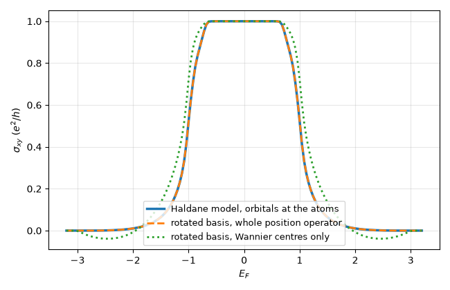
full position operator: largest deviation 3.9e-12
centres only: largest deviation 0.20
Total running time of the script: (0 minutes 0.445 seconds)