
Note
Go to the end to download the full example code.
Every State in an Energy Window: Spectrum Slicing#
A dense diagonalization gives every eigenstate of a flake, at a cost
\(O(N^3)\) and \(N^2\) numbers in memory: 32 GB of complex
numbers for 45,000 sites. Shift-invert (get_eig_sparse())
gives the few states nearest one energy. Between the two, one often
wants all the states in a window: those near a Dirac point, inside a
gap, or in one band.
get_eig_window() gets them by spectrum
slicing. The number of eigenvalues below an energy \(\sigma\) is
exact and cheap, by Sylvester’s law of inertia: the sparse factorization
\(P(H-\sigma)P^T = LDL^\dagger\) has as many negative pivots as
\(H\) has eigenvalues below \(\sigma\). The window is bisected
until each slice holds at most n_slice eigenvalues, and each slice
is solved by shift-invert Lanczos about its centre. The count tells the
solver how many eigenpairs it must return, which makes the method
reliable: Lanczos alone can miss copies of a degenerate level, and the
missing ones are found by deflation (shift-invert with the eigenvectors
already found projected out).
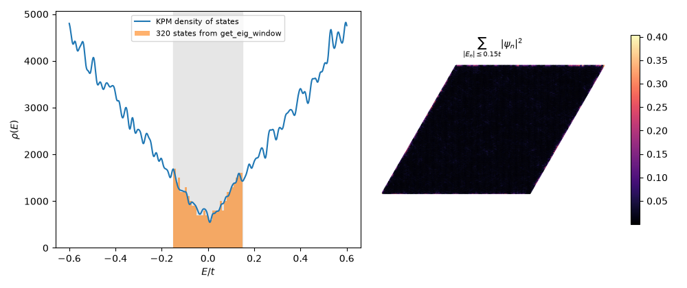
Here: graphene flakes with Anderson disorder \(W = t\). On a small
flake the window agrees with the dense spectrum. On a flake of 28,800
sites the number of states in \(|E| \le 0.15t\) agrees with the
density of states of the kernel polynomial method
(tbkit.kpm.dos()), and the states weigh more than three times as
much near the edges as their share of the sites: graphene’s zigzag
edges carry states at \(E = 0\).
import time

import numpy as np
import matplotlib.pyplot as plt
from scipy.integrate import trapezoid

import tbkit.kpm as kpm
import tbkit.lattices as lattices
from tbkit.system import System


def flake(n, w=1., seed=1):
    lat = lattices.honeycomb()
    lat.get_lattice(n, n)
    sys = System(lat)
    sys.set_hopping([{'n': 1, 't': -1.}])
    sys.set_onsite({'a': 0., 'b': 0.})
    np.random.seed(seed)
    sys.set_onsite_dis(w)
    sys.get_ham()
    return sys


e_min, e_max = -0.15, 0.15
A small flake: the window against the dense spectrum#
small = flake(24)
small.get_eig()
dense = small.en[(small.en >= e_min) & (small.en <= e_max)]
small.get_eig_window(e_min, e_max, eigenvec=True, n_slice=10)
ham = small.ham.toarray()
print('{} sites: {} states in the window, max |E - E_dense| = {:.1e}'.format(
    small.lat.sites, len(small.en), np.max(np.abs(small.en - dense))))
assert len(small.en) == len(dense) and np.allclose(small.en, dense, atol=1e-10)
assert np.allclose(ham @ small.rn, small.rn * small.en, atol=1e-9)
assert np.allclose(small.rn.conj().T @ small.rn, np.eye(len(small.en)), atol=1e-9)
1152 sites: 21 states in the window, max |E - E_dense| = 8.6e-15
28,800 sites#
large = flake(120)
start = time.perf_counter()
large.get_eig_window(e_min, e_max, eigenvec=True)
elapsed = time.perf_counter() - start
residual = np.max(np.linalg.norm(large.ham @ large.rn - large.rn * large.en, axis=0))
print('{} sites: {} states in the window in {:.1f} s, max residual {:.1e}'.format(
    large.lat.sites, len(large.en), elapsed, residual))
assert residual < 1e-8
assert np.allclose(large.rn.conj().T @ large.rn, np.eye(len(large.en)), atol=1e-8)

# the same count from the kernel polynomial method, without any eigenstate
energies = np.linspace(-0.6, 0.6, 601)
e_grid, rho = kpm.dos(large.ham, n_moments=2048, n_random=20, e_grid=energies, seed=0)
inside = (e_grid >= e_min) & (e_grid <= e_max)
kpm_count = trapezoid(rho[inside], e_grid[inside])
print('KPM estimate: {:.0f} states'.format(kpm_count))
assert abs(kpm_count / len(large.en) - 1) < 0.05

# the states near E = 0 live on the zigzag edges
coor = large.lat.coor
weight = large.intensity.sum(axis=1)
edge = (coor['x'] < coor['x'].min() + 2.) | (coor['x'] > coor['x'].max() - 2.) \
    | (coor['y'] < coor['y'].min() + 2.) | (coor['y'] > coor['y'].max() - 2.)
share = weight[edge].sum() / weight.sum()
print('weight within 2 bonds of the edges: {:.0%} (they hold {:.0%} of the sites)'.format(
    share, edge.mean()))
assert share > 3 * edge.mean()
28800 sites: 320 states in the window in 14.6 s, max residual 8.3e-15
KPM estimate: 313 states
weight within 2 bonds of the edges: 10% (they hold 3% of the sites)
fig, (ax1, ax2) = plt.subplots(1, 2, figsize=(10, 4.2))
ax1.plot(e_grid, rho, color='C0', label='KPM density of states')
ax1.hist(large.en, bins=30, range=(e_min, e_max), weights=np.full(len(large.en), 30 / (e_max - e_min)),
         color='C1', alpha=0.6, label='{} states from get_eig_window'.format(len(large.en)))
ax1.axvspan(e_min, e_max, color='0.9', zorder=0)
ax1.set_xlabel(r'$E/t$')
ax1.set_ylabel(r'$\rho(E)$')
ax1.legend(fontsize=8)
sc = ax2.scatter(coor['x'], coor['y'], c=weight, s=0.3, cmap='magma', rasterized=True)
ax2.set_aspect('equal')
ax2.set_title(r'$\sum_{|E_n| \leq 0.15t} |\psi_n|^2$', fontsize=10)
ax2.axis('off')
fig.colorbar(sc, ax=ax2, shrink=0.8)
fig.tight_layout()
plt.show()
Total running time of the script: (0 minutes 21.090 seconds)