
Note
Go to the end to download the full example code.
Second-Order Optical Conductivity from Three-Index Chebyshev Moments#
A crystal without inversion symmetry answers a field \(\mathbf{E}(\omega_1) + \mathbf{E}(\omega_2)\) with a current at \(\omega_1 + \omega_2\), \(j^a = \sigma^{abc}(\omega_1, \omega_2)E^b(\omega_1)E^c(\omega_2)\): second-harmonic generation at \(\omega_1 = \omega_2\), and at \(\omega_2 = -\omega_1\) a direct current, the shift current of The Bulk Photovoltaic Effect: the Shift Current of Gapped Graphene.
tbkit.kpm.nonlinear_optical_conductivity() computes the whole
tensor for a sample with no Brillouin zone, as KITE’s
conductivity_optical_nonlinear. The field enters through the Peierls
phases (the velocity gauge), \(H(\mathbf{A}) = H + A_bh^b +
\frac12A_bA_ch^{bc} + \dots\), whose derivatives \(h^{b\dots}\) come
from finite_derivatives(). The density matrix
to second order is a sum of traces such as
\(\mathrm{Tr}[\delta(\varepsilon-H)\,h^aG^R(\varepsilon+\omega_3)\,h^b
G^R(\varepsilon+\omega_2)\,h^c]\), which the kernel polynomial method
expands in the three-index moments
\(\mathrm{Tr}[T_m(\tilde H)h^aT_n(\tilde H)h^bT_p(\tilde H)h^c]\).
Two checks:
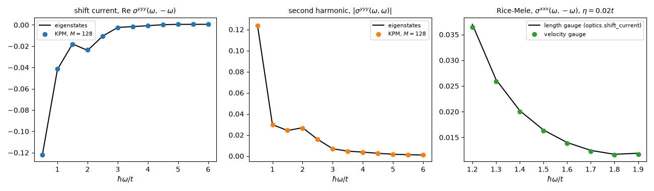
On a small torus of gapped graphene with the exact trace, the Chebyshev series against the sum over eigenstates of the same density matrix, written out below: shift current and second harmonic. With the broadening \(\eta = 0.5t\) and \(M = 128\) moments the error, about \((\pi a/M\eta)^2\) (\(2a\) the spectral width), is a few percent.
In the tight-binding basis the velocity gauge is exact: as \(\eta \to 0\) it gives the length-gauge shift conductivity of
tbkit.optics.shift_current()(Sipe and Shkrebtii), here on the Rice-Mele chain, whose shift current has a closed form (Fregoso, Morimoto and Moore 2017).
import numpy as np
import matplotlib.pyplot as plt
import scipy.linalg as LA

import tbkit.kpm as kpm
import tbkit.models as models
import tbkit.optics as optics
from tbkit.kspace import KSpace
from tbkit.lattice import Lattice


def sum_over_states(ham, der, component, w1, w2, eta, area):
    r'''
    sigma^abc(w1, w2) from the eigenstates: rho_1 = [h^c, f] / (w2 + i eta - E_nm),
    rho_2 = ([h^b, rho_1] + [h^bc, f]/2) / (w1 + w2 + 2 i eta - E_nm),
    j^a = -Tr[rho_2 h^a + rho_1 h^ab + f h^abc / 2] / area (charge -e),
    and A_b A_c = -E_b E_c / (w1 w2), symmetrized in (b, w1) <-> (c, w2).
    '''
    en, vec = LA.eigh(ham)
    f = (en < 0.).astype(float)
    h = {k: vec.conj().T @ v @ vec for k, v in der.items()}
    fmn, enm = f[None, :] - f[:, None], en[:, None] - en[None, :]

    def key(*letters):
        return ''.join(sorted(letters))

    def response(a, b, c, o1, o2):
        rho1 = h[c] * fmn / (o2 + 1j * eta - enm)
        rho2 = (h[b] @ rho1 - rho1 @ h[b] + h[key(b, c)] * fmn / 2) / (o1 + o2 + 2j * eta - enm)
        return (np.sum(rho2 * h[a].T) + np.sum(rho1 * h[key(a, b)].T)
                + np.sum(f * np.diag(h[key(a, b, c)]).real) / 2)

    a, b, c = component
    return (response(a, b, c, w1, w2) + response(a, c, b, w2, w1)) / (2 * area * w1 * w2)
Gapped graphene: Chebyshev moments against the eigenstates#
A staggered potential \(\pm0.4t\) breaks inversion and opens a gap \(0.8t\); the mirror \(x \to -x\) leaves \(\sigma^{yyy} = -\sigma^{yxx}\) and \(\sigma^{xxx} = 0\).
hbn = models.haldane(t1=1., t2=0., M=0.4)
n, eta = 6, 0.5
area = n * n * optics.cell_area(hbn)
ham = hbn.finite_ham(n, periodic=True, sparse=True)
der = hbn.finite_derivatives(n, 'yyy', periodic=True, sparse=True)
dense = {k: v.toarray() for k, v in der.items()}
omega = np.linspace(0.5, 6., 12)

shift = kpm.nonlinear_optical_conductivity(ham, der, omega, -omega, 'yyy', eta=eta, n_moments=128,
                                           n_random=None, area=area)
shg = kpm.nonlinear_optical_conductivity(ham, der, omega, omega, 'yyy', eta=eta, n_moments=128,
                                         n_random=None, area=area)
shift_exact = np.array([sum_over_states(ham.toarray(), dense, 'yyy', w, -w, eta, area) for w in omega])
shg_exact = np.array([sum_over_states(ham.toarray(), dense, 'yyy', w, w, eta, area) for w in omega])
print('largest relative error: shift {:.1%}, second harmonic {:.1%}'.format(
    np.max(np.abs(shift / shift_exact - 1)), np.max(np.abs(shg / shg_exact - 1))))
assert np.all(np.abs(shift / shift_exact - 1) < 0.06)
assert np.all(np.abs(shg / shg_exact - 1) < 0.06)
# a direct current: real, for a linear polarization in a time-reversal-symmetric crystal
assert np.all(np.abs(shift_exact.imag) < 1e-12 * np.abs(shift_exact.real).max())

der_x = hbn.finite_derivatives(n, 'yxx', periodic=True, sparse=True)
shift_yxx = kpm.nonlinear_optical_conductivity(ham, der_x, omega[:4], -omega[:4], 'yxx', eta=eta,
                                               n_moments=128, n_random=None, area=area)
assert np.allclose(shift_yxx, -shift[:4], atol=1e-10)
largest relative error: shift 2.2%, second harmonic 3.3%
Velocity gauge and length gauge#
The Rice-Mele chain of Fregoso, Morimoto and Moore (the ‘b’ site at
half the cell, hoppings \((t\pm\delta)/2\), onsite \(\pm m\)),
stacked along \(y\) without coupling, as
shift_current() takes 2D models. A ring of 400 cells
and \(\eta = 0.02t\): the two gauges agree to the order of
\(\eta\), away from the edges of the absorption band, where the
Lorentzian and Gaussian broadenings of the van Hove singularities differ.
t, delta, m = 1., 0.4, 0.3
lat = Lattice(unit_cell=[{'tag': 'a', 'r0': (0., 0.)}, {'tag': 'b', 'r0': (0.5, 0.)}],
              prim_vec=[(1., 0.), (0., 1.)])
rm = KSpace(lat)
rm.set_hopping([{'i': 0, 'j': 1, 'R': (0, 0), 't': (t + delta) / 2},
                {'i': 1, 'j': 0, 'R': (1, 0), 't': (t - delta) / 2}])
rm.set_onsite({'a': m, 'b': -m})
cells = 400
ham_rm = rm.finite_ham((cells, 1), periodic=True)
der_rm = rm.finite_derivatives((cells, 1), 'xxx', periodic=True)
omega_rm = np.linspace(1.2, 1.9, 8)  # inside the band, away from its edges at 1.0 and 2.09
eta_rm = 0.02
velocity = np.array([sum_over_states(ham_rm, der_rm, 'xxx', w, -w, eta_rm, cells) for w in omega_rm]).real
length = optics.shift_current(rm, omega_rm, eta=eta_rm, nk=(20000, 1))
print('velocity / length gauge: {:.3f} to {:.3f}'.format(np.min(velocity / length), np.max(velocity / length)))
assert np.all(np.abs(velocity / length - 1) < 0.02)
velocity / length gauge: 0.984 to 0.988
fig, (ax1, ax2, ax3) = plt.subplots(1, 3, figsize=(13, 3.8))
ax1.plot(omega, shift_exact.real, 'k-', label='eigenstates')
ax1.plot(omega, shift.real, 'o', color='C0', label='KPM, $M = 128$')
ax1.set_title(r'shift current, Re $\sigma^{yyy}(\omega, -\omega)$', fontsize=10)
ax2.plot(omega, np.abs(shg_exact), 'k-', label='eigenstates')
ax2.plot(omega, np.abs(shg), 'o', color='C1', label='KPM, $M = 128$')
ax2.set_title(r'second harmonic, $|\sigma^{yyy}(\omega, \omega)|$', fontsize=10)
ax3.plot(omega_rm, length, 'k-', label='length gauge (optics.shift_current)')
ax3.plot(omega_rm, velocity, 'o', color='C2', label='velocity gauge')
ax3.set_title(r'Rice-Mele, $\sigma^{xxx}(\omega, -\omega)$, $\eta = 0.02t$', fontsize=10)
for ax in (ax1, ax2, ax3):
    ax.set_xlabel(r'$\hbar\omega/t$')
    ax.legend(fontsize=8)
fig.tight_layout()
plt.show()
Total running time of the script: (0 minutes 30.221 seconds)